
Journal of Environment Protection and Sustainable Development, Vol. 1, No. 4, September 2015 Publish Date: Aug. 12, 2015 Pages: 193-202
Uncertainty Analysis and Modelling of Phytoplankton Dynamics in Coastal Waters
Lixia Niu1, *, P. H. A. J. M. Van Gelder2, Yiqing Guan3, J. K. Vrijling1
1Department of Hydraulic Engineering, Delft University of Technology, Delft, the Netherlands
2Department of Safety and Security Science, Delft University of Technology, Delft, the Netherlands
3Department of Hydrology and Water Resources, Hohai University, Nanjing, China
Abstract
As the most important indicator of the coastal ecosystem, phytoplankton plays an important role in the whole impact-effect chain. The present study aims to investigate the characteristics of phytoplankton dynamics using an ecological model of BLOOM II (one module of the Delft3D suite), and to give insight in the predictions with an integration of uncertainty analysis. The comparisons of the model output and the observations demonstrate that the BLOOM II model is able to reproduce the reliable levels of the phytoplankton biomass (in terms of chlorophyll a) and the associated environmental variables (nutrients and suspended matter). Compared with nitrogen, phosphorus is less sensitive to the phytoplankton biomass. The Gamma distribution can fit with the values of the phytoplankton biomass regardless of the observations, the model output in the surface layer, and the depth-averaged values. Pay particular attention to the depth-averaged chlorophyll a, the model output varies from 4.80 mg m-3 to 17.33 mg m-3. With respect to uncertainty arising from the model itself, the prediction with uncertainty analysis ranges from 8.00 mg m-3 to 15.27 mg m-3 within the 95% confidence interval, with a Monte Carlo error of 0.03 mg m-3.
Keywords
BLOOM II, Phytoplankton Biomass, Chlorophyll a, Uncertainty Analysis, Frisian Inlet
Received: July 4, 2015
Accepted: July 27, 2015
Published online: August 11, 2015
@ 2015 The Authors. Published by American Institute of Science. This Open Access article is under the CC BY-NC license. http://creativecommons.org/licenses/by-nc/4.0/
Contents
1. Introduction 2. Methodology and Materials 2.1. Data Information 2.2. BLOOM II Model 2.3. Uncertainty Analysis 3. Results 3.1. Observational Analysis 3.2. Estimate of the Phytoplankton Growth Rate 3.3. Validation of the BLOOM II Model 3.4. Model Output 3.5. Uncertainty Analysis 4. Discussion Acknowledgement
1. Introduction
The coastal ecosystem is facing a big challenge caused by the effects of anthropogenic activities and coastal development (Conley et al., 2002; Andersen, 2006). As the indicator of the coastal ecosystem, phytoplankton plays an important role in the whole impact-effect chain and is responsible for most of primary production. The investigation of phytoplankton dynamics has provided useful insights and a better understanding of the coastal ecosystem.
Phytoplankton dynamics (i.e. growth, loss, grazing, biomass, bloom) causes changes with the characteristics of the environmental variables in the water column (Pedersen and Borum, 1996; Mei et al., 2002; Recknagel et al., 2006; Taylor and Ferrari, 2011). The associated environmental variables are divided into three categories: physical condition, chemical condition and biological condition. Take the physical condition as an example to illustrate the relations with phytoplankton dynamics: temperature and light intensity are closely linked with the phytoplankton growth (Eppley, 1972; Smith, 1980; Geider et al., 1997, 1998; Ornolfsdottir et al., 2004); a change of salinity has an effect on the phytoplankton community (Schmidt, 1999; Lionard et al., 2005); wind stress and tidal currents affect the turbulent mixing rate, determining the vertical distributions of the phytoplankton biomass (Serra et al., 2007; Wong et al., 2007; Woernle et al., 2014) and affecting the species composition due to the effects on the availability of light intensity and nutrients (Ferris and Christian, 1991); suspended matter absorbs and scatters light intensity, implying that the phytoplankton is limited by light availability in the high turbidity zone (Allen et al., 2002). Of all the environmental factors, phytoplankton dynamics is mainly refined by the limitations of light and nutrient availability (Cloern, 1987; Eilers and Peeters, 1988; Boyer et al., 2009; Swart et al., 2009).
However, measuring in situ properties of the phytoplankton is a time consuming and expensive task. As such, the mathematical models become useful tools to perform the investigation based on the limited number of observations. Evans and Parslow (1985) present a model to explain the annual cycle of the phytoplankton population. Steele and Henderson (1992) elucidate that the plankton models depend on both the form of the mortality closure and the parameter estimation. Skogen et al. (1995) use a coupled three-dimensional physical-chemical-biological ocean model to study the primary production. Los and Wijsman (2007), Los et al. (2008), Los (2009), Blauw et al. (2009), and Niu et al. (2015) develop the ecological model of BLOOM II/GEM to investigate the phytoplankton processes in coastal waters.
In this study, the BLOOM II model (one module of the Delft3D suite) is introduced to investigate the phytoplankton variability at the Frisian Inlet located in the north of the Netherlands (figure 1), Lauwersoog and Huibertgat as the proxies to explain the phytoplankton variability. With the well-known simplification of the model, the predictions over a certain area and a certain time have a large uncertainty. Stressing the uncertainty arising from the model, the Bayesian Markov Chain Monte Carlo (BMCMC) simulation is approached to give insight in the model output with uncertainty analysis within the 95% confidence interval.
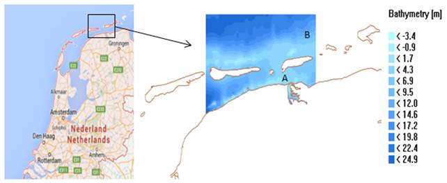
Figure 1. Location map of the Frisian Inlet and surrounding water zones, A: Lauwersoog station, B: Huibertgat station.
2. Methodology and Materials
2.1. Data Information
The water environment in this area is favourable for the phytoplankton (Van Beusekom et al., 2012). Seven variables (chlorophyll a, ![]() , mg m-3; nitrate,
, mg m-3; nitrate, ![]() , mg l-1; ammonium,
, mg l-1; ammonium, ![]() , mg l-1; phosphorus,
, mg l-1; phosphorus, ![]() , mg l-1; silicate,
, mg l-1; silicate, ![]() , mg l-1; suspended matter,
, mg l-1; suspended matter, ![]() , mg l-1;salinity, PSU) over the year of 2009, measured either biweekly or monthly, are collected from the main database of DONAR (accessible through http://www.eea.europa.eu/data-and-maps/data/external/donar-historical-water-measurement-data ). Another three variables of light intensity (
, mg l-1;salinity, PSU) over the year of 2009, measured either biweekly or monthly, are collected from the main database of DONAR (accessible through http://www.eea.europa.eu/data-and-maps/data/external/donar-historical-water-measurement-data ). Another three variables of light intensity (![]() , W m-2), water temperature (
, W m-2), water temperature (![]() , 0C) and wind profile (speed: m s-1, direction: degree), measured daily, are collected from the KNMI database (accessible through www.knmi.nl). Note that the variables of
, 0C) and wind profile (speed: m s-1, direction: degree), measured daily, are collected from the KNMI database (accessible through www.knmi.nl). Note that the variables of![]() ,
, ![]() , and wind profile are set as domain parameters, while the others are site-specific. Various studies have completely accepted that chlorophyll a can be a reliable estimate of the phytoplankton biomass (Voros and Padisak, 1991; Scharler and Baird, 2003; Boyer, et al., 2009), which is also the focus in this study.
, and wind profile are set as domain parameters, while the others are site-specific. Various studies have completely accepted that chlorophyll a can be a reliable estimate of the phytoplankton biomass (Voros and Padisak, 1991; Scharler and Baird, 2003; Boyer, et al., 2009), which is also the focus in this study.
2.2. BLOOM II Model
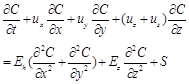
The BLOOM II model has been well applied in the Dutch coast, the Wadden Sea, and the North Sea (Blauw and Los, 2004; Los et al., 2008; Blauw et al., 2009; Los, 2009; Niu et al., 2015). As one module of the Delft3D suite, the BLOOM II model can simulate the phytoplankton processes, the nutrient cycling, and the transport of the substances. This model can be applied in any water systems. The detailed information of the BLOOM II model can be found after Los (2009). The main governing equation can be explained by the advection-diffusion equation, written as:
 (1)
(1)
In which, ![]() denotes the concentration of the substance;
denotes the concentration of the substance; ![]() ,
, ![]() , and
, and ![]() denote the velocity in the
denote the velocity in the ![]() -,
-, ![]() -, and
-, and ![]() -direction;
-direction; ![]() denotes the sinking velocity;
denotes the sinking velocity; ![]() denotes the horizontal turbulent diffusivity;
denotes the horizontal turbulent diffusivity; ![]() denotes the vertical turbulent diffusivity;
denotes the vertical turbulent diffusivity; ![]() denotes the sources of mass.
denotes the sources of mass.
The BLOOM II model is coupled with the hydrodynamic conditions (i.e. velocity, water level, salinity, sediment, wind stress, tidal currents, vertical eddy viscosity, and vertical eddy diffusivity) calculated in the Delft3D-FLOW module. In the set-up of the hydrodynamic model in this case, 85×77 grids are generated. For the vertical dimension, the water column is subdivided into 10 layers using a sigma-coordinated approach. While in the set-up of the BLOOM II model, three layers are integrated: surface layer, middle layer, and bottom layer.
2.3. Uncertainty Analysis
The classic modelling approaches are processed with some simplifications, but the actual processes are not deterministic in the presence of uncertainty. The object has three possible values: original and original ±uncertainty. The uncertainties, arising from input parameters, model itself, and model scenarios, cannot be avoided in any of the analyses. For example, we stress the significance of the phytoplankton in this study, and the grazing rate of the zooplankton is considered as a constant value. However, the grazing process of the zooplankton is sensitive to the analysis of the phytoplankton, actually varied with the environmental factors (Steele and Henderson, 1992; Haney and Jackson, 1996). Therefore, the simplification of the model is accompanied with an overestimate or underestimate of the real state. The BMCMC simulation, a full description of the uncertainty, is approached to integrate the uncertainty analysis, processed with the WinBugs (accessible through http://www.mrc-bsu.cam.ac.uk/software/bugs/).
Bayesian inference accesses to the quantification and propagation of uncertainty via a probability, in light of the known information of the object.
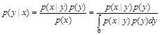 (2)
(2)
In which, ![]() denotes the known information;
denotes the known information; ![]() denotes the unknown information;
denotes the unknown information; ![]() denotes the prior distribution;
denotes the prior distribution; ![]() denotes the likelihood function;
denotes the likelihood function; ![]() denotes the posterior distribution.
denotes the posterior distribution.
Markov Chain Monte Carlo is a general method to compute the posterior distribution. With the commonly used algorithm, Gibbs Sampler, the Bayesian Markov Chain Monte Carlo simulation has been widely applied to describe the uncertainty (Kuczera, 1999; Kelly and Smith, 2009; Niu et al., 2015).
3. Results
3.1. Observational Analysis
The statistics of the observed variables at the Frisian Inlet are shown in table 1. At Lauwersoog station, chlorophyll a fluctuates around a big interval, 0.64-87.89 mg m-3, with the mean value of 26.92 mg m-3 and the standard deviation of 25.1 mg m-3. The minimum chlorophyll a appears on the day of 18th May and the maximum appears on the day of 17th April. The nutrients show a similar pattern in the entire Frisian Inlet, increasing since winter but decreasing quickly in spring. The nitrate ranges from 0.01 mg l-1 to 0.53 mg l-1, while 0.005-0.520 mg l-1 for ammonium, 0.013-0.14 mg l-1 for phosphorus and 0.03-1.42 mg l-1 for silicate. Most of the ratios of ![]() are lower than the optimal condition of 16:1 (Brzezinski, 2004), which indicates a nitrogen deficiency relative to the phosphorus. At Huibertgat station, chlorophyll a varies from 1.11 mg m-3 to 124 mg m-3, with the mean value of 12.07 mg m-3 and the standard deviation of 25.67 mg m-3. The minimum appears on the day of 20th February and the maximum appears on the day of 20th April. The concentrations of the nutrients are lower than that at Lauwersoog station. It is to infer that the phosphorus limits the phytoplankton growth from November to March because the ratios of
are lower than the optimal condition of 16:1 (Brzezinski, 2004), which indicates a nitrogen deficiency relative to the phosphorus. At Huibertgat station, chlorophyll a varies from 1.11 mg m-3 to 124 mg m-3, with the mean value of 12.07 mg m-3 and the standard deviation of 25.67 mg m-3. The minimum appears on the day of 20th February and the maximum appears on the day of 20th April. The concentrations of the nutrients are lower than that at Lauwersoog station. It is to infer that the phosphorus limits the phytoplankton growth from November to March because the ratios of ![]() are larger than the optimal condition during that time period.
are larger than the optimal condition during that time period.
The phytoplankton biomass is not a single factor but as a consequence of many environmental variables. The contributions of the associated variables are shown in table 2. The phytoplankton biomass (in terms of chlorophyll a) is significantly correlated with suspended matter (![]() =0.6,
=0.6, ![]() <0.01), and is moderately correlated with silicate, ammonium, and light intensity (|
<0.01), and is moderately correlated with silicate, ammonium, and light intensity (|![]() |>0.3,
|>0.3, ![]() <0.05), in which, silicate and ammonium denote the negative contributions. The random effects of the variables are also taken into account using the Bootstrap method, based on 500 random samples.
<0.05), in which, silicate and ammonium denote the negative contributions. The random effects of the variables are also taken into account using the Bootstrap method, based on 500 random samples.
Table 1. Statistics of the observed variables at the Frisian Inlet over the year of 2009.
| Variables | Lauwersoog station | Huibertgat station | ||||||
| Min | Max | Mean | SD | Min | Max | Mean | SD | |
|
| 0.64 | 87.89 | 26.92 | 25.1 | 1.11 | 124 | 12.07 | 25.67 |
|
| 0.01 | 0.53 | 0.15 | 0.16 | 0.01 | 0.72 | 0.19 | 0.2 |
|
| 0.005 | 0.52 | 0.147 | 0.16 | 0.005 | 0.3 | 0.08 | 0.08 |
|
| 0.013 | 0.14 | 0.051 | 0.03 | 0.008 | 0.043 | 0.021 | 0.01 |
|
| 0.03 | 1.42 | 0.47 | 0.4 | 0.01 | 0.9 | 0.28 | 0.27 |
|
| 0.22 | 21.6 | 7.41 | 6.8 | 1.35 | 51.43 | 14.1 | 14.28 |
|
| 27 | 390 | 105 | 77.3 | 3.6 | 37 | 17.6 | 8.79 |
| Salinity | 25.9 | 31.7 | 29.56 | 1.81 | 27.4 | 31.9 | 30.2 | 1.35 |
|
| 4.51 | 354.63 | 123.5 | 97.3 | ||||
|
| 2.1 | 19.8 | 11.27 | 5.59 | ||||
| Wind speed (m s-1) | 0.2 | 13.1 | 5.38 | 2.55 | ||||
*. Min indicates the minimum value;
*. Max indicates the maximum value;
*. SD indicates the standard deviation.
Table 2. Correlation analysis between the phytoplankton biomass (in terms of chlorophyll a) and other environmental forces, determined by the observations in 2009.
| Salinity | Wind | |||||||||||
|
| Pearson Correlation ( | -.243 | -.194 | -.443* | -.527* | -.171 | .593** | .534* | .195 | -.333 | ||
| Sig. (2-tailed) ( | .289 | .399 | .044 | .014 | .459 | .005 | .013 | .396 | .140 | |||
| Bootstrapc | Bias | .037 | .025 | -.013 | -.015 | -.004 | -.035 | .006 | .011 | -.006 | ||
| Std. Error | .266 | .226 | .136 | .100 | .168 | .222 | .128 | .169 | .146 | |||
| 95% Confidence Interval | Lower | -.699 | -.550 | -.695 | -.719 | -.468 | -.022 | .258 | -.129 | -.606 | ||
| Upper | .322 | .360 | -.168 | -.326 | .214 | .872 | .774 | .526 | -.054 | |||
*. Correlation is significant at the 0.05 level (2-tailed).
**. Correlation is significant at the 0.01 level (2-tailed).
c. Unless otherwise noted, bootstrap results are based on 500 bootstrap samples.
3.2. Estimate of the Phytoplankton Growth Rate
The commonly used estimate of the growth rate is as the functions of temperature, light intensity and nutrients (Eppley, 1972; Smith, 1980; Geider et al., 1997, 1998; Ornolfsdottir et al., 2004; Bissinger and Montagnes, 2008). In this study, we integrate the growth-temperature function into the light curve.
The phytoplankton growth rate presents a seasonal variation, increasing gradually since the winter time, reaching the peak values in the summer days and then decreasing till the winter. Normally, the maximum growth rate is around 2.0 day-1 in coastal waters (Bowie et al., 1985; Arhonditsis and Brett, 2005). In this case, the maximum growth rate is 1.87 day-1 appeared on the day of 18th August and the minimum is 0.38 day-1 appeared on the day of 6th March.
3.3. Validation of the BLOOM II Model
Prior to the application of the BLOOM II model, it is necessary to question whether the model is reliable in this case. In this validation section, the graphical view of the comparisons between the model outputs and the observations is displayed in figure 2 and figure 3, involved six variables (![]() ,
,![]() ,
,![]() ,
,![]() ,
,![]() , and
, and ![]() ) at two stations (Lauwersoog and Huibertgat). The comparisons demonstrate that the BLOOM II model can reproduce reliable predictions of the phytoplankton biomass (in terms of chlorophyll a), nutrients, and suspended matter at the Frisian Inlet.
) at two stations (Lauwersoog and Huibertgat). The comparisons demonstrate that the BLOOM II model can reproduce reliable predictions of the phytoplankton biomass (in terms of chlorophyll a), nutrients, and suspended matter at the Frisian Inlet.
3.4. Model Output
In view of the specific demand, the phytoplankton species can be distinguished by the classification of Margalef (1978): the order of vertical turbulent diffusivity and nutrient availability. Thus, dinoflagellates and diatoms are equally significant at Lauwersoog station, while diatoms are the dominant species at Huibertgat station.
The annual variations of the phytoplankton biomass and the associated variables are derived in the different water layers at the Frisian Inlet. Chlorophyll a is largely varied between the layers, while small variations of other variables appear within the layers. The increase of chlorophyll a is followed by a decrease of nutrients, excluding the trend of![]() .
.
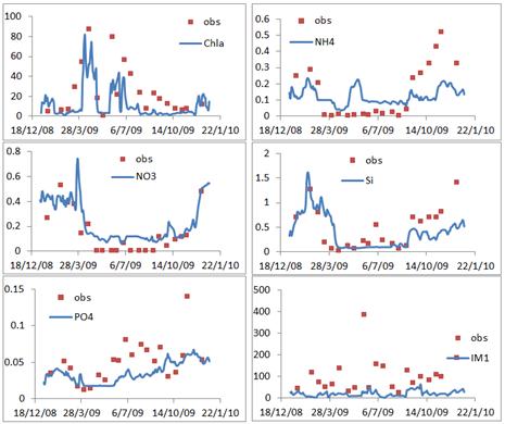
Figure 2. Graphical view of the comparisons between the observations (the red scatters) and the model outputs (the blue smooth lines) at Lauwersoog station over the year of 2009, confined in the surface layer.
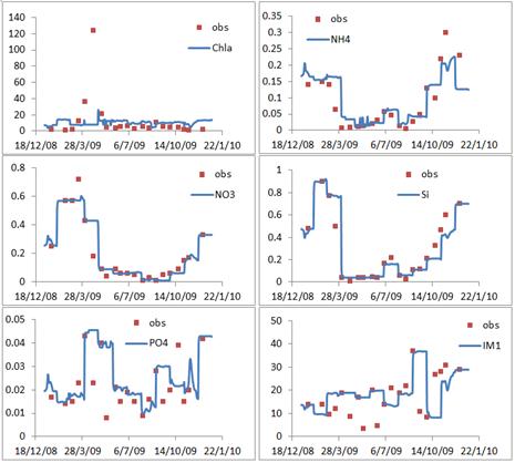
Figure 3. Graphical view of the comparisons between the observations (the red scatters) and the model outputs (the blue smooth lines) at Huibertgat station over the year of 2009, confined in the surface layer.
The previous section has presented the model outputs in the surface layer (the blue smooth lines in the figure 2 and figure 3). Take Huibertgat station as an example to describe the variations of the variables. Chlorophyll a varies from 3.85 mg m-3 to 26.18 mg m-3, with the mean value of 10.30 mg m-3 and the standard deviation of 2.79 mg m-3. The maximum value appears on the day of 1st May and the minimum appears on the day of 13th January. The ammonium varies from 0.011 mg l-1 to 0.292 mg l-1, with the mean value of 0.098 mg l-1 and the standard deviation of 0.067 mg l-1. The nitrate ranges from 0.010 mg l-1 to 0.602 mg l-1, with the mean value of 0.218 mg l-1 and the standard deviation of 0.200 mg l-1. The phosphorus ranges from 0.009 mg l-1 to 0.045 mg l-1, with the mean value of 0.025 mg l-1 and the standard deviation of 0.010 mg l-1. The silicate ranges from 0.040 mg l-1 to 0.921 mg l-1, with the mean value of 0.322 mg l-1 and the standard deviation of 0.298 mg l-1. The suspended matter varies from 8.230 mg l-1 to 36.888 mg l-1, with the mean value of 18.925 mg l-1 and the standard deviation of 7.601 mg l-1. Higher values of nitrogen and silicon appear in February and March.
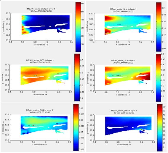
Figure 4. Annual-averaged distributions of phytoplankton biomass (in terms of chlorophyll a) and water properties in the surface layer at the Frisian Inlet over the year of 2009.
Figure 4 displays the annual-averaged distributions of the variables in the entire Frisian Inlet, confined in the surface layer. Higher values of chlorophyll a appear in the west zone, accompanied with a similar trend of ![]() and an opposite pattern of
and an opposite pattern of ![]() . Compared with
. Compared with ![]() , other nutrients have a relative small range. Most of chlorophyll a distributes at a range of [10,11] mg m-3, while [0.11, 0.14] mg l-1 for
, other nutrients have a relative small range. Most of chlorophyll a distributes at a range of [10,11] mg m-3, while [0.11, 0.14] mg l-1 for ![]() , [0.25, 0.30] mg l-1 for
, [0.25, 0.30] mg l-1 for ![]() , [0.30, 0.35] mg l-1 for
, [0.30, 0.35] mg l-1 for ![]() , [0.04, 0.045] mg l-1 for
, [0.04, 0.045] mg l-1 for ![]() , and [16,18] mg l-1 for
, and [16,18] mg l-1 for ![]() . The relationships between chlorophyll a and other variables coincide with the observational analysis. Among the nutrients,
. The relationships between chlorophyll a and other variables coincide with the observational analysis. Among the nutrients, ![]() is the most sensitive parameter to chlorophyll a, followed by the importance of
is the most sensitive parameter to chlorophyll a, followed by the importance of ![]() . Meanwhile,
. Meanwhile, ![]() has a close link with chlorophyll a, a lower chlorophyll a corresponding to a higher
has a close link with chlorophyll a, a lower chlorophyll a corresponding to a higher ![]() .
.
Particular attention is paid to the depth-averaged distribution of chlorophyll a, varying from 4.801 mg m-3 to 17.337 mg m-3, with the mean value of 11.334 mg m-3 and the standard deviation of 1.874 mg m-3. Considering the random effects, the Bootstrap method is used, displayed in table 3. The mean value of chlorophyll a ranges from 11.137 mg m-3 to 11.519 mg m-3 within the 95% confidence interval, with a bias of -0.001 mg m-3 and a standard error of 0.097 mg m-3. The standard deviation of chlorophyll a varies from 1.715 mg m-3 to 2.030 mg m-3 within the 95% confidence interval, with a bias of -0.006 mg m-3 and a standard error of 0.081 mg m-3. The statistics of the depth-averaged nutrients and suspended matter have a reliable range within the 95% confidence interval. In addition, the Gamma distribution can fit with chlorophyll a regardless of the observations, the model outputs in the surface layer, and the depth-averaged values, displayed in figure 5.
3.5. Uncertainty Analysis
Simplification of the model must be accompanied with uncertainty. The BMCMC simulation is used to describe the uncertainty and to give insight in the model output with uncertainty analysis. The object is the depth-averaged phytoplankton biomass (in terms of chlorophyll a). Prior to the approaching of the BMCMC simulation in this case, the convergence is required to be tested. Figure 6 displays the statistics of the BMCMC simulation, including the widely used Gelman-Rubin convergence test and the density of the phytoplankton biomass with uncertainty. Two chains are designed in this case, and 2000 random samples are distributed to each chain. The rule of the convergence in the Gelman-Rubin test is to make the red line tended to 1. The prediction with uncertainty analysis varies from 8.006 mg m-3 to 15.27 mg m-3 within the 95% confidence interval, with a Monte Carlo error of 0.031 mg m-3. Figure 7 shows the completely trace plots of the phytoplankton biomass (in terms of chlorophyll a), based on 4000 samples.
Table 3. Statistics of the depth-averaged variables at the Frisian Inlet over the year of 2009.
| Depth-averaged | Statistic | Bootstrap | ||||
| Bias | Std. Error | 95% Confidence Interval | ||||
| Lower | Upper | |||||
|
| Mean | 11.334 | -0.001 | 0.097 | 11.137 | 11.519 |
| SD | 1.877 | -0.006 | 0.081 | 1.715 | 2.030 | |
| Skewness | -0.487 | 0.003 | 0.157 | -0.768 | -0.160 | |
|
| Mean | 0.096 | 0.000 | 0.003 | 0.089 | 0.103 |
| SD | 0.066 | 0.000 | 0.001 | 0.063 | 0.068 | |
| Skewness | 0.233 | -0.002 | 0.097 | 0.052 | 0.419 | |
|
| Mean | 0.219 | 0.000 | 0.011 | 0.197 | 0.240 |
| SD | 0.201 | 0.000 | 0.005 | 0.189 | 0.210 | |
| Skewness | 0.701 | 0.003 | 0.099 | 0.509 | 0.895 | |
|
| Mean | 0.026 | 0.000 | 0.001 | 0.025 | 0.027 |
| SD | 0.011 | 0.000 | 0.000 | 0.010 | 0.011 | |
| Skewness | 0.652 | 0.000 | 0.094 | 0.483 | 0.835 | |
|
| Mean | 0.324 | 0.000 | 0.016 | 0.292 | 0.353 |
| SD | 0.298 | -0.001 | 0.008 | 0.281 | 0.313 | |
| Skewness | 0.709 | -0.001 | 0.098 | 0.533 | 0.904 | |
|
| Mean | 19.076 | 0.017 | 0.379 | 18.333 | 19.850 |
| SD | 7.648 | -0.021 | 0.285 | 7.050 | 8.202 | |
| Skewness | 0.823 | -0.006 | 0.071 | 0.686 | 0.963 | |
*. Unless otherwise noted, bootstrap results are based on 1000 bootstrap samples
*. The object of the 95% confidence interval in the Bootstrap method is the estimate, like mean value, standard deviation, and skewness.
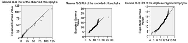
Figure 5. Gamma distribution fit with the phytoplankton biomass (in terms of chlorophyll a), involving the observations, the modelled chlorophyll a in the surface layer, and the depth-averaged values.
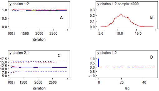
Figure 6. Statistics of the BMCMC simulation. A: the Gelman-Rubin convergence test; B: the density of the phytoplankton biomass (in terms of chlorophyll a); C: the quantiles of the phytoplankton biomass (in terms of chlorophyll a), including the 2.5%, the median, and the 97.5%; D: the autocorrelation function.
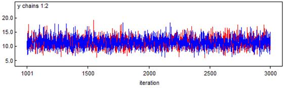
Figure 7. Trace plots of the prediction with uncertainty analysis (in terms of chlorophyll a) at the Frisian Inlet over the year of 2009, based on 4000 random samples and expressed in mg m-3. The red line indicates chain 1, and the blue line indicates chain 2.
4. Discussion
In order to better understand the coastal ecosystem, an ecological model of BLOOM II, widely applied to a range of water systems, is proposed in this case based on the limited number of observations. Graphical view of the comparisons between the model output and the observations demonstrates that the BLOOM II model can reproduce reliable predictions in this case (figure 2 and figure 3): five programme for the parameter calibration (![]() ,
,![]() ,
,![]() ,
,![]() , and
, and ![]() ) and one programme for the model validation (chlorophyll a).
) and one programme for the model validation (chlorophyll a).
In this case, there is a low vertical mixing rate due to the semi-enclosed position (figure 1). The slow exchange between the tidal inlet and the North Sea also increases the water residence time, which promotes the phytoplankton growth. The characteristics of the phytoplankton biomass are derived in the different water layers. In the surface layer, the chlorophyll a varies around a big range, 3.85-26.18 mg m-3. Higher values appear in spring, followed by a rapid reduction of the nutrients. There is a small variation between the middle layer and the bottom layer. In another words, the water column can be subdivided into two layers: surface layer and bottom layer. With the random effects, the value of the object is not deterministic but a reliable range. For the depth-averaged chlorophyll a, the mean value varies from 11.13 mg m-3 to 11.52 mg m-3 within the 95% confidence interval, and the standard deviation varies from 1.71 mg m-3 to 2.03 mg m-3 (table 3).
To stress the uncertainty of the model output, the Bayesian Markov Chain Monte Carlo simulation is approached to get insight in the prediction with uncertainty analysis. The modelled depth-averaged chlorophyll a varies from 4.80 mg m-3 to 17.34 mg m-3, with the mean value of 11.33 mg m-3 and the standard deviation of 1.874 mg m-3. While the new prediction of chlorophyll a fluctuates from 8.01 mg m-3 to 15.27 mg m-3 within the 95% confidence interval, with a MC error of 0.03 mg m-3, based on 4000 random samples.
The findings of this research are expected to provide valuable information for the coastal ecosystem management. More observed environmental factors are needed to improve the prediction, like the biological properties and the chemical conditions.
Acknowledgement
The authors would like to thank the Rijkswaterstaat (accessible through http://www.eea.europa.eu/data-and-maps/data/external/donar-historical-water-measurement-data ) and the KNMI (accessible through www.knmi.nl) for providing the data. The authors also thank the anonymous reviewers.
References
- Allen K.W., Lane A., and Tett P., 2002. Phytoplankton, sediment and optical observations in Netherlands coastal water in spring. Journal of Sea Research, 47, 303-315.
- Andersen J.H., Schluter L., and Aertebjerg G., 2006. Coastal eutrophication: recent developments in definitions and implications for monitoring strategies. Journal of Plankton Research, 28, 621-628.
- Arhonditsis G.B. and Brett M.T., 2005. Eutrophication model for lake Washington (USA), Part I. Model description and sensitivity analysis. Ecological modelling, 187, 140-178.
- Bissinger J.E., Montagnes J.S., Sharples J., and Atkinson D., 2008. Predicting marine phytoplankton maximum growth rates from temperature: improving on the Eppley curve using quantile regression. Limnol. Oceanogr., 53, 487-493.
- Blauw A. and F.J. Los, 2004.Analysis of the response of phytoplankton indicators in Dutch coastal waters to nutrient reduction scenarios, WL| Delft Hydraulics, report Z3844.
- Blauw A., F.J. Los, M. Bokhorst and L.A. Erftemeijer, 2009.GEM: a generic ecological model for estuaries and coastal waters. Hydrobiologia, 618: 175-198.
- Bowie G.L., Mills W.B., Porcella D.B., Campbell C.L., Pagenkopf J.R., Rupp G.L., Johnson K.M., Chan P.W.H., and Gherini S.A., 1985. Rates constants and kinetics formulations in surface water quality modelling (second edition). Rep.EPA 600/3-85/40, US.EPA, Athens, Georgia, pp455.
- Boyer J.N., Kelble C.R., Ortner P.B., and Rudnick D.T., 2009. Phytoplankton bloom status: chlorophyll a biomass as an indicator of water quality condition in the southern estuaries of Florida, USA. Ecological indicators, 95, s56-s67.
- Brzezinski M.A., 2004. The Si:C:N ratio of marine diatoms: interspecific variability and the effect of some environmental variables. Journal of Phycology, 21, 347-357.
- Cloern J.E., 1987. Turbidity as a control on phytoplankton biomass and productivity in estuaries. Continental shelf research, 7, 1367-1381.
- Conley, D. J., Markager, S., and Andersen, J. et al., 2002. Coastal eutrophication and the Danish National Aquatic Monitoring and Assessment Program. Estuaries, 25, 706–719.
- Eilers P.H.C. and J.C.H. Peeters, 1988. A model for the relationship between light intensity and the rate of photosynthesis in phytoplankton. Ecological modelling, 42, 199-215.
- Eppley R.W., 1972. Temperature and phytoplankton growth in the sea. Fishery Bulletin, 70, 1063-1085.
- Evans G.T. and Parslow J.S., 1985. A model of annual plankton cycles. Biological Oceanography, 3, 327-347.
- Ferris, J. M. and Christian, R., 1991. Aquatic primary production in relation to microalgal responses to changing light: a review. Aquatic Sciences, 53(2):187-217.
- Geider R.J., Maclntyre H.L., and Kana T.M., 1997. Dynamic model of phytoplankton growth and acclimation: responses of the balanced growth rate and the chlorophyll a: carbon ratio to light, nutrient-limitation and temperature. Marine Ecology Progress Series, 148, 187-200.
- Geider R.J., Maclntyre H.L., and Kana T.M., 1998. A dynamic regulatory model of phytoplanktonic acclimation to light, nutrients, and temperature. Limnol. Oceanogr., 43, 679-694.
- Haney J.D., and Jackson G.A., 1996. Modeling phytoplankton growth rates. Journal of Plankton Research, 18, 63-85.
- Kelly D.L. and Smith C.L., 2009. Bayesian inference in probabilistic risk assessment- the current state of the art. Reliability engineering and system safety, 94, 628-643.
- Kuczera G., 1999. Comprehensive at-site flood frequency analysis using Monte Carlo Bayesian inference. Water Resources Research, 35: 1551-1557.
- Lionard M., Muylaert K., van Gansbeke D., and Vyverman W., 2005.Influence of changes in salinity and light intensity on growth of phytoplankton communities from the Scheldt river and estuary (Belgium/The Netherlands). Hydrobiologia, 540, 105-115.
- Los F. J. and J. W. M. Wijsman, 2007. Application of a validated primary production model (BLOOM) as a screening tool for marine, coastal and transitional waters. Journal of Marine Systems, 64: 201–215.
- Los F.J., M.T.Villars and M.W.M.Van der Tol, 2008. A 3-dimensional primary production model (BLOOM/GEM) and its applications to the (southern) North Sea (coupled physical-chemical-ecological model). Journal of Marine System. Vol 74: 259-294.
- Los F.J., 2009. Eco-hydrodynamic modelling of primary production in coastal waters and lakes using BLOOM. Thesis, Wageningen University, ISBN 978-90-8585-329-9.
- Margalef R., 1978. Life-form of phytoplankton as survival alternatives in an unstable environment. Oceanologica Acta, 1, 493-509.
- Mei Z.P., Legendre L., Gratton Y., Tremblay J.E., LeBlanc B., Mundy C.J., Klein B., Gosselin M., Larouche P., Papakyriakou T.N., Lovejoy C., and von Quillfeldt C.H., 2002. Physical control of spring-summer phytoplankton dynamics in the North Water, April-July 1998. Deep-Sea Research II, 49, 4959-4982.
- Niu L., Van Gelder P.H.A.J.M., Guan Y., Zhang C. and Vrijling J.K., 2015.Probabilistic analysis of phytoplankton biomass at the Frisian Inlet (NL). Estuarine, Coastal and Shelf Science, 155, 29-37.
- Ornolfsdottir E.B., Lumsden S.E., and Pinckney J.L., 2004. Nutrient pulsing as a regulator of phytoplankton abundance and community composition in Galveston Bay, Texas. Journal of Experimental Marine Biology and Ecology, 303, 197-220.
- Pedersen M.F., and Borum J., 1996. Nutrient control of algal growth in estuarine waters. Nutrient limitation and the importance of nitrogen requirements and nitrogen storage among phytoplankton and species of macroalgae. Marine Ecology Progress Series, 142, 261-272.
- Rechnagel F., Talib A., and van der Molen D., 2006.Phytoplankton community dynamics of two adjacent Dutch lakes in response to seasons and eutrophication control unravelled by non-supervised artificial neural networks. Ecological Informatics, 1, 277-285.
- Scharler U.M. and D.Baird, 2003. The influence of catchment management on salinity, nutrient stoichiometry and phytoplankton biomass of Eastern Cape estuaries, South Africa. Estuarine, Coastal and Shelf Science, 56, 735-748.
- Schmidt I., 1999. The importance of phytoplankton biomass as an ecosystem parameter in shallow bays of the Baltic. I. Relationships between biomass and system characteristics. Limnologica, 29, 301-307.
- Serra T., Vidal J., Casamitjana X., Soler M., and Colomer J., 2007.The role of surface vertical mixing in phytoplankton distribution in a stratified reservoir. Limnology Oceanography, 52, 620-634.
- Skogen M.D., Svendsen E., Berntsen J., Aksnes D. and Ulvestad K.B., 1995.Modelling the primary production in the North Sea using a coupled three-dimensional physical-chemical-biological ocean model. Estuarine, coastal and shelf science, 41, 545-565.
- Smith R.A., 1980. The theoretical basis for estimating phytoplankton production and specific growth rate from chlorophyll, light and temperature data. Ecological Modelling, 10, 243-264.
- Steele J.H. and Henderson E.W., 1992. The role of predation in plankton models. Journal of Plankton Research, 14, 157-172.
- Swart R.J., Biesbroek G.R., Binnerup S., Carter T.R., Henrichs T., and Loquen S., et al., 2009.Europe adapts to climate change: comparing national adaptation strategies (No. 01/2009). Finnish Environment Institute (SYKE), Helsinki.
- Taylor, J.R. and Ferrari, R., 2011. Shutdown of turbulent convection as a new criterion for the onset of spring phytoplankton blooms. Limnology and Oceanography, 56, 2293–2307.
- Van Beusekom J.E.E., Christian Buschbaum and Karsten Reise, 2012.Wadden Sea tidal basins and the mediating role of the North Sea in ecological processes: scaling up of management? Ocean & Coastal Management, 68, 69-78.
- Voros L. and Padisak J., 1991. Phytoplankton biomass and chlorophyll a in some shallow lakes in central Europe.Hydobiologia, 215, 111-119.
- Woernle L.H., Dijkstra H.A., and van der Woerd H.J., 2014.Sensitivity of phytoplankton distributions to vertical mixing along a North Atlantic transect. Ocean Science, 10, 993-1011.
- Wong K.T.M., Lee J.H.W. and Hodgkiss I.J., 2007. A simple model for forecast of coastal algal blooms. Estuarine, Coastal and Shelf Science, 74, 175-196.


