
American Journal of Information Science and Computer Engineering, Vol. 2, No. 5, September 2016 Publish Date: Oct. 5, 2016 Pages: 63-69
Fault Prediction Method Combining Principal Component Analysis and Back Propagation Neural Network
Kaixuan Wang1, Mei Li1, *, Wanxin Shi1, Xu Liu1, Shiyao Qin2, Xiaojing Ma2
1School of Information Engineering, China University of Geosciences, Beijing, China
2New Energy Institute, China Electric Power Research Institute, Beijing, China
Abstract
Fault prediction of wind turbine could greatly reduce its operation and maintenance cost. A fault prediction method combining Principal Component Analysis (PCA) and Back Propagation Neural Network (BPNN) is proposed. Using only BPNN to predict the turbine fault, one has to pick out proper attributes for training and that can be a troublesome work. With PCA revealing the hidden relationship between attributes, we no longer need to select attributes by experience thus saving cost. Also, PCA largely reduce the dimension of attributes so that the curse of dimensionality can be avoided. The proposed PCA-BPNN method can improve the accuracy by 3% compared BPNN method, so that abnormal state of the mechanical faults can be determined more precisely, again reduce the maintenance cost.
Keywords
Fault Prediction, Data Mining, Principal Component Analysis, Back Propagation Neural Network, Wind Turbine
Received: September 8, 2016
Accepted: September 18, 2016
Published online: October 5, 2016
@ 2016 The Authors. Published by American Institute of Science. This Open Access article is under the CC BY license. http://creativecommons.org/licenses/by/4.0/
Contents
1. Introduction 2. Methods 2.1. The Principal Component Analysis (PCA) 2.2. The Error Back Propagation Neural Network Algorithm 3. Experiments and Result 3.1. BPNN Method with 38 Attribute 3.2. BPNN Method with 9 Attribute 3.3. PCA-BPNN Method 4. Discussion 4.1. D-value and Turbine Fault 4.2. PCA-BPNN Method and BPNN Method Comparison 5. Conclusions Acknowledgement
1. Introduction
The market forecasts that by 2018 the wind energy cumulative gigawatts (GW) will be 43% higher than of 2015's GW [1]. For wind turbines the maintenance costs are high because of their remote location, and this can amount to as much as 25 to 30% of the total energy production [2]. The most effective way to reduce maintenance costs is to continuously monitor generators’ status and predict the malfunction of wind turbine. Then the system degradation problems can be found and responded in time. Maintenance can be carried out ahead of time before the system crash and excess maintenance is avoided. Therefore, fault prediction could maximize the normal production of wind power plant and greatly reduce maintenance costs.
The main methods of wind turbine fault diagnosis include these types such as the fault mode analysis based on statistical data, the fault diagnosis based on time series prediction, model-based fault diagnosis of control system, the fault diagnosis based on vibration analysis, and other auxiliary diagnosis methods like acoustic emission technique and ultrasonic capacitance liquid level detection [3, 4]. These methods did not combine different characteristic data such as vibration, power, start stop record, which could be more informative.
Up to now, as more and more monitoring data, e.g. the temperature data, the driving power, the swing in the direction of the tower, the average wind speed, the angle of blade and the average generator speed are available, many data mining methods are utilized in fault prediction, for instance, graphical model-based approach proposed by Aloraini A and Sayed-Mouchaweh M [5], SVM-based solution by Santos P et al. [6], GA optimization method by Odofin Sarah et al. [7] and Neural Network used by Lan Q et al. [8] probabilistic neural network by Malik H and Mishra S [9], k-means and neural network by Xu Liu et al. [10]. These methods mainly focus on predicting directly with original data or data selected by experience instead of preprocessing data. Take BPNN as a sample. The researchers always input original data or select the data by experience. It leads to an inefficient data analysis because of the redundancy of data or unrevealed internal relationship of the data.
The proposed method in this paper aims to reduce the redundancy of the attributes by utilizing PCA to preprocess the data. After that, a part of those data are used to train the BPNN and the rest of the data are predicted. The D-value of the actual value and the predicted value indicates the symptom of fault. The experiment led up to the fact that the prediction accuracy can be actually improved with the principal component analysis method.
2. Methods
2.1. The Principal Component Analysis (PCA)
PCA is a dimension reduction method based on statistical analysis [11, 12]. Assume that there are n samples and every sample has p attributes. They form a n×p data matrix as following.
 (1)
(1)
We note a column vector of X as ![]()
![]() . When the original attributes are large, we have to replace them with a few mutually orthogonal comprehensive components. The new column vector is respectively called the first, second… m-th principal component, and represents new attributes that has the largest variance in order.
. When the original attributes are large, we have to replace them with a few mutually orthogonal comprehensive components. The new column vector is respectively called the first, second… m-th principal component, and represents new attributes that has the largest variance in order.
 (2)
(2)
Where is the eigenvector corresponding to the i-th eigenvalue by quantity of matrix X’s covariance matrix or correlation matrix. There are six steps to achieve principal components.
Step 1. The data which are n samples with attributes form a matrix with column vectors.
Step 2. Each element of matrix subtracts the mean of its column.
Step 3. Compute the covariance matrix of the above matrix.
Step 4. Calculate the eigenvalues and eigenvectors of the covariance matrix.
Step 5. Rank the eigenvalues from the highest to the lowest in order to choose the top corresponding m eigenvectors. The rest eigenvectors are dropped.
Step 6. Calculate the m principal components according to formula (2).
The typical goal of a PCA is to reduce the dimensionality of the original feature space by projecting it onto a smaller subspace, where the eigenvectors will form the axes. The eigenvectors with the lowest eigenvalues bear the least information about the distribution of the data.
2.2. The Error Back Propagation Neural Network Algorithm
The BPNN algorithm is extensively used in prediction. It is expert in approximating any nonlinear function, so it is especially suitable for the issues of complex internal mechanism. Its self-learning ability and parallel fast computation also make it practical. Generally, the BPNN has two stages, training and testing.
During the training phase, training data including the input and the expected output are given to the neutral network. For example, the input might be an encoded picture of an animal, and the output could be a code that represents the category of the animal. Figure 1 shows the topology of the BPNN that includes an input layer, one hidden layer and an output layer. It should be noted that it can have more than one hidden layer.
Suppose there are D inputs, K outputs, M hidden layer nodes. are the input variables, are the hidden layer’s variables, and are the output variables, and are the weight parameters between and, and. and are the bias vectors of the hidden layer nodes and the output layer nodes.
Figure 1. Three-layer neural network.
Take node as example. Its output is and its bias is, which is one conponent of bias vector. Its output is determined by its bias, the outputs of its former layer nodes and its activation function.
![]() (3)
(3)
![]() (4)
(4)
where f is the activation function and it is usually the sigmoid function ![]() .
.
The expected output is then compared with the actual output value, and an error signal is computed.
 (5)
(5)
The training stage is a learning process and composed of two steps, which are input signal forward propagation and error signal back propagation. When the error exceeds its allowable scope, the BPNN will change over to the error signal back propagation step. The output error signals are transmitted backwards from the nodes of the output layer to each node in the immediate hidden layer to modify their connection weights and the bias of the nodes of the output layer proportion to the error signal, partial derivative of the output node activation function and the output of the connected node, where![]() is the learning rate.
is the learning rate.
![]() (6)
(6)
The variation ![]() is calculated as follows.
is calculated as follows.
 (7)
(7)
This mechanism is also applied to its bias and the weights and biases of hidden layer nodes. There are five steps in the training stage.
Step 1. An input sample is applied to the input layer.
Step 2. The signal propagates layer by layer through the hidden layers until an output is produced according to formula (3) and (3).
Step 3. For each of the output nodes, the actual output value is compared with the expected output according to formula (5).
Step 4. Modify the weights and the bias of each node according to formula (6) and (7).
Step 5. The learning process will keep working and the above steps repeat for every input samples until the total error of the output of the network gradually reduced to the degree that can be accepted or to the set number of learning.
3. Experiments and Result
The proposed method has been tested on the wind turbine gearbox bearing condition monitoring using MATLAB. Among all wind turbine faults, gearbox bearing faults are relatively common [1, 3]. When the gearbox is out of order, it’s bearing temperature would arise. Thus among the numerous parameters contained by wind turbine status data, the gearbox bearing temperature is the predicted target. The data was provided by New Energy Institute of China Electric Power Research Institute, from March 17 to April 17 in 2015, taking one month every 10 minutes to log data for test, with a total of 4500 data points.
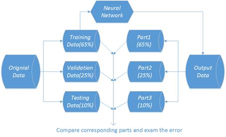
Figure 2. Data partion for training validation and testing.
The data was separated into 3 parts, first 65% of data for Neural Network training, next 25% for validation and last 10% for testing as figure 2 shows. The actual temperature will rise when wind turbine faults. We define D-value here to determine wind turbine fault (discussed in detail in part 4.1). Let Ta= actual gearbox oil temperature, Tb= predict gearbox oil temperature
D-value =Ta-Tb (8)
The fault happened after data point 4430, i.e. in the testing dataset. So unlike most of the prediction problem, we are expecting the predict value not fitting the actual ones in the testing set. The prediction accuracy we be represent by the mean square error of the validation set.
3.1. BPNN Method with 38 Attribute
Figure 3 shows the last 1000 point of actual and predicted value of gearbox bearing temperature applying BPNN method with 38 attribute. The prediction result fit very well but the fault data was also tracked, the D-value is small all the time in this case we can’t tell the turbine fault.
3.2. BPNN Method with 9 Attribute
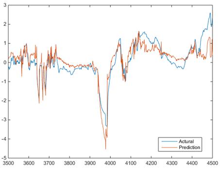
Because too much features can lead to data overfit when applying BPNN, we selected 9 attributes of wind turbines, part of them are listed in Table 1. And the BPNN prediction result is shown Figure 4 (a), with the blue line representing the actual gearbox bearing temperature and orange for prediction value. Compared to Figure 3, the prediction is less accurate but in the last about 80 point the prediction line deviate from the actual one obviously, also see figure 4 (b) the D-value rise indicates turbine fault.
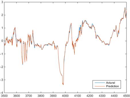
Figure 3. Actual and predicted value of gearbox bearing temperature applying BPNN method with 38 attribute.
(a)
(b)
Figure 4. (a) Actual and predicted value of gearbox bearing temperature applying BPNN method with 38 attribute (b) the corresponding D-value.
Table 1. Part of normalized data of 9 attributes of wind turbines selected by experience*.
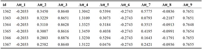
* Att_1: Swing amplitude of driving chain [%]; Att_2: Ambient temperature [°C]; Att_3: Variable plasma motor temperature [°C] Att_4: Cabin temperature [°C]; Att_5: Active power [kW]; Att_6: Swing amplitude of drive direction tower [%]; Att_7: mean wind speed [m/s]; Att_8: angle of Blade 1 [°]; Att_9: Generator mean speed [rpm];
3.3. PCA-BPNN Method
Selecting attributes by experience is sometimes a troublesome work, but with PCA we can avoid selecting features by hand. The main difference between our proposed PCA-BPNN method and BPNN method is that we are now running PCA to all attribute to reduce the dimensions before sending data to the neural net. We employ PCA to reduce the dimension, but it is notable that generally we calculate the variance to decide how many dimension we want. One commonly use value is variance=0.95 meaning that 95% of the information of the original data is retained. The PCA process tells that with 7 new features we achieve 0.95 variance as shown in figure 5.
By setting variance we can decide which dimension to reduce to. Setting variance to 0.95 in fact reduce the dimension to 7 as in figure 5, by engineer experience we choose 9 features to make prediction. The number of features are relatively close, showing the effectiveness of PCA process in another way.
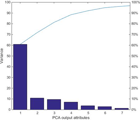
Figure 5. Variance of each new feature adding up to 0.95.
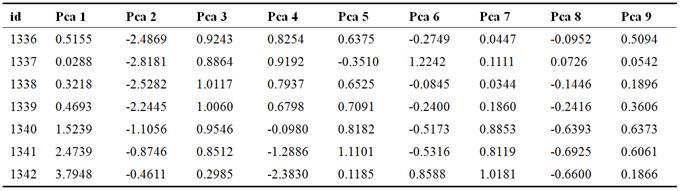
Table 2. Part of PCA process output data by setting variance=0.95.
The prediction alone with the actual value are shown in figure 6 (a), if no fault occurs i.e. before about point 4430 that prediction is closer to the actual, and when fault happens the two lines obviously separated. Also see figure 6 (b) the overall fluctuation is smaller than that in figure 4 (b) which mean less prediction error.
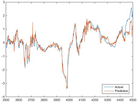
(a)
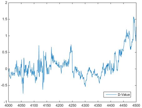
(b)
Figure 6. (a) Actual and predicted value of gearbox bearing temperature applying PCA- BPNN method (b) the corresponding D-value.
4. Discussion
4.1. D-value and Turbine Fault
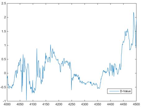
Using steady state working D-Value of proposed PCA-BPNN method, we set four warning lines as in figure 7. The red line and purple line stands for upper and lower bound of temperature respectively, if the D-value keeps exceeding for a set time, the machine will halt. The orange line and light blue green are used for warning, notify people earlier before the turbines have fault. We can find the D-value goes beyond the up or down alarm line for several times, this are some impulses which disappear quickly so that the alarm won’t be triggered.
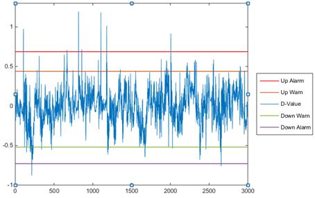
Figure 7. Using steady state working D-value to set warning lines.
Put the four warning together with the last 500 point in figure 8, we can see that the D-value keeps exceeding the up alarm line after point 4430, thus the fault can successfully be predicted with PCA-BPNN method.
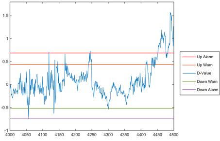
Figure 8. D-value and fourcritical line for fault warning.
4.2. PCA-BPNN Method and BPNN Method Comparison
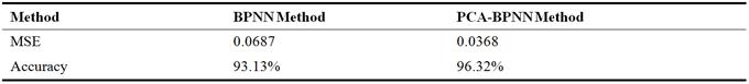
For Xi represent the actual temperature of i-th point and Yi for the prediction, the MSE is calculated by the formula (8). Note again that we do not use the MSE of prediction result because our test data set contains the fault data and that will affect the result. The MSE and corresponding accuracy are listed in table 3, compared to BPNN method, PCA-BPNN increase the accuracy by 3%.
Table 3. CV MSE of two different experiment.
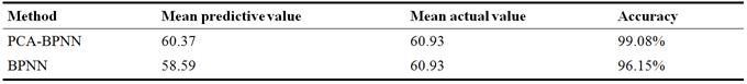
Also we can see in table 4 that the prediction accuracy increased by about 3% from 96.15% to 99.08% with respect to the mean predictive value and mean actual value, just like that of MSE value.
Table 4. Mean predictive value of two different experiment.
5. Conclusions
According to the results of data comparison, it can be seen that the prediction given by PCA-BPNN method is closer to the actual values than that without using PCA. The forecast error is smaller and most important, no need to select attributes by experience. The PCA-BPNN method can improve the learning accuracy at about 3% and promote the timeliness of the machine fault diagnosis. Combining PCA and neural network is efficient to pick up representative attributes of samples thus realize the redundancy reduction of attributes. That is, to achieve better operation and maintenance effects, the prediction accuracy of the proposed method is better than that of the neural network algorithm, it is more timely and accurate to determine the abnormal condition of the gearbox. The method can also be extended to the operation and maintenance of other machine faults, which has good practical value.
Acknowledgement
This work was financially supported by the National Natural Science Foundation of China (Grant No. 41572347 and Grant No. 41374185).
The authors appreciate the support of Jinqiao Seed Fund of Beijing Association of Science and Technology.
References
- Azevedo D; Machado H D; Araújo, et al. A review of wind turbine bearing condition monitoring: State of the art and challenges. RSER, 2016, 56:368-379.
- Aziz, M. A.; Noura, H., & Fardoun, A. General review of fault diagnostic in wind turbines. 18th Mediterranean Conf. on Con. & Aut., 2010, MED’10, pp.1302 - 1307 doi: 10.1109/med.2010.5547870.
- Amirat Y, Benbouzid MEH, Al-Ahmar E, Bensaker B and Turri S. A brief status on condition monitoring and fault diagnosis in wind energy conversion systems. RSER, 2009, 13, pp.2629-36.
- Schlechtingen M, Santos IF and Achiche S. Wind turbine condition monitoring based on SCADA data using normal behavior models. Part 1: System description. App. Soft Com. 2013, vol. 14, pp.447–460.
- Aloraini, A., & Sayed-Mouchaweh, M. Graphical Model Based Approach for Fault Diagnosis of Wind Turbines. International Conference on Machine Learning and Applications,2014, pp.614 - 619.
- Santos P; Villa LF; Reñones A; Bustillo A and Maudes J. An SVM-Based Solution for Fault Detection in Wind Turbines. Sensors, 2015, vol.15, 5627-48.
- Odofin S, Gao Z and Sun K. Robust fault estimation in wind turbine systems using GA optimisation. Industrial Informatics (INDIN), 2015 IEEE 13th International Conference on. IEEE, 2015, pp. 580-5.
- Lan Q; Zhao PD; Wang ML. Fault Diagnosis of Wind Turbines Based on Improved Neural Network. Advanced Materials Research, Trans Tech Publ, 2014, pp. 78-83.
- Malik H; Mishra S. Application of Probabilistic Neural Network in Fault Diagnosis of Wind Turbine Using FAST, TurbSim and Simulink. Procedia Computer Science. 2015; vol.58, pp.186-93.
- Xu Liu, Mei Li et al, A Predictive Fault Diagnose Method of Wind Turbine Based on K-means Clustering and Neural Networks. JIT, 2016, vol.17(online), doi: 10.6138/JIT.2016.17.7.20151027i.
- Jolliffe I. Principal component analysis. Wiley Online Library, 2002.
- Mcmurtrey SD. Training and optimizing distributed neural networks using a genetic algorithm. Nova Southeastern University, 2010.


