Stochastic Mathematical Model of "Tunnelling" ― Penetration of Particle Through Prohibitive Barrier

Vladimir A. Dobrynskii^*

Institute for Metal Physics of N.A.S.U., Kiev, Ukraine

Abstract

In the article, properties of solutions to one specific kind stochastic ordinary differential equation system are examined. This system simulates the Brownian walks which active particles make along the-axis due to the permanent white noise action. In order to study the system solution properties, a number of snapshots of experimental 1-dimensional frequency distribution function that is build up on base of the found solutions is made. Watching these snapshots we find that there exists a parameter domain such that the system under study can serve as a mathematical model of process of tunnelling ― a penetration of elementary particle through a prohibitive potential barrier.

Keywords

Active Particle, Vivacity, Natural Internal Frequency, Tunnel Effect, Penetration

Received:June 15, 2016
Accepted: July 1, 2016
Published online: August 5, 2016

@ 2016 The Authors. Published by American Institute of Science. This Open Access article is under the CC BY license. http://creativecommons.org/licenses/by/4.0/

1. Introduction

In the elementary particle physics, there is the elementary particle "tunnelling" phenomenon, i.e. its penetration through a prohibitive potential barrier. Since the given phenomenon in its nature is statistical, obviously that it is impossible to build up a deterministic mathematical model of this phenomenon. Therefore, one should concentrate efforts on search of its stochastic mathematical model. In doing so first what should be taken into account is that the particles in nature possess certain properties that vary in process of their interaction with the medium, where they are contained. In other words, these particles are "active" by their own nature as against the "passive" ones which have no such the kind properties at all. It is plain that this "activity" must certainly be reflected in any model that is proposed to consideration. Second, it is clear also that the active particles interact with the external medium, so say, "actively" in the sense that the interaction process consists in varying of both the properties of particles that undergo action of the external medium on ones and the properties of the medium itself to resist to movement of the particles. The latter ones are modifying in the course of time due to the aforesaid interaction too. Taking into account these circumstances it is plain that creating of a stochastic mathematical model of the aforementioned phenomenon one should reflect in the model the "activity" of its particles by means of introducing of parameters and variables which must describe the active properties of the particles. (On existence of such kind the particle characteristics one could guess observing results of simulation of the Brownian particle walk dynamics of the stochastic mathematical model that are presented in the next section.)

In what follows, we consider the simplest such kind model. It includes one active parameter (the particle "natural internal frequency") and one active variable (the particle "vivacity") only. As a reader can be convinced later oneself a presence of such the kind parameters and variables allows single selected active particles to visit space domains which are closed for the passive (usual) ones can never visit the aforesaid domains.

As a whole a problem of how determinism and chance interplay each other in nature phenomena stays one of the most important fundamental questions standing in front of science up till now. Widespread systematic investigations directed to research the given problem are started recently relatively. In doing so random walk researching is making both in random and non-random environments [1]. Investigations showed to researchers’ surprise that a stochastic action of random noise stabilizes behaviour of system dynamics rather than insets chaos inside it very often [2-4]. There are a lot of references (see, e.g., [5-7]), where influence of noise on the particles dynamics and their Brownian random walk are studied. Methods used for solving and simulating of solutions to the stochastic differential equations which model random processes are permanently developed [8-12]. However one aspect of the problem ― what is a sort of particles which the noise acts on, ― as far as we know, was never considered early. As it is easily see from observation and comparing of their histograms for experimental 1-dimensional frequency distribution function, the active particles and passive ones give a very distinct different response on the white noise action.

Our approach to studying of the Brownian walk dynamics of the active particles that undergo a persistent action of the standard white noise consists in simulation of this dynamics with aid of two stochastic ordinary differential equations and, in general, goes on the studies in [13-15].

2. Mathematical Model

For creating the mathematical model of the particles dynamics, it is assumed that i) they do not interact each other and ii) dynamics of all particles controls by the same stochastic ordinary differential equations. In order to reduce a quantity of numerical computations and to simplify analysis of results of numerical experiments, we restrict ourselves with considering of the simplest among the others model. Therefore, in the model under creature, (ϊ) a dimension of space where the particles make their Brownian walk is equal to 1, (ϊϊ) there are two only space parameter that provide influence the space on the particles, one of which describes an "observable " (friction-like) interaction particles with space and the other may provide the "hidden" accumulation of one only specific (energy-like) particle characteristic, and (ϊϊϊ) changing of the aforesaid particle characteristic value depends on both the "observable" and "hidden" interaction of the particles with the space. A concrete form of the expressions using for creating of the model under study is borrowed from [13-15]. In there, the similar model is used for simulation of the Brownian walk of the oscillator in plane with non-linear non-homogeneous friction. Anyway we research numerically solutions of the following system of stochastic ordinary differential equations:

,    (1)

.

Here  be the space particle co-ordinate, be its vivacity, , and  be its natural internal frequency. By  is denoted the total instantaneous stochastic force acting on the particle at time . This is the Gaussian white noise with correlations giving by its first and second: ,) moments respectively. (For generating of such the kind noise, the standard Wiener’s process is used usually.) The particle is called active when and passive otherwise, i.e. when . All parameters are constants. In doing so ,,. As for , then it is supposed always that . Considering Eq. (1) in detail it is not difficult to analyse qualitatively how varying of different parameters influence on dynamics of the Brownian particle walk. Such a kind analysis is done in [13-14] for the system similar to Eq. (1) although different. So, it is stated there the parameters like ,are paired in a sense that simultaneous identical increasing of them does in general not change dynamics of the random particle walk qualitatively. Increasing one of them, say,  results in suppressing of the random walk and, on the contrary, increasing of  leads to its wide-spreading. Thus, in order to balance contribution of  and  in dynamics of solution to Eq. (1) one should take their values identical, say, equal to 1. The physical significance of  and  is a general level of the space interaction with the particles and a maximal power of the white noise influence on the particles respectively. By the same manner, one can study the rest of parameters and estimate their influence on dynamics of the Brownian particle walk. Consider, for instance, , the coefficient of non-linearity of the space resistance to the particles movement. It is evident that the more the value of  the higher the friction barrier rises in the positive half-axis and the less the space friction to the particle displacement in the negative one. As for the watching of phenomenon of the active particle penetration over the prohibitive friction barrier, it is clear that, in order to have a possibility to observe this phenomenon, the value of must be balanced with , the particle start point coordinate. Really, the aforementioned phenomenon is, as we shall see further, a result of long-time evolution of the well-developed Brownian walk of the particles. It is evident that if the particles start in the closest barrier vicinity, one can then obtain such the kind well-developed Brownian walk only in the end of its very-very long evolution. On the contrary, if the start point is removed too far away from the barrier to the left, then the Brownian walk dynamics of the particle can develop so stormy that will lead to underflow/overflow and, as a consequence, will not give a possibility to watch the aforementioned phenomenon. Thus, the values of and are paired in the sense that they have to be balanced too, etc. A propos, in [13-14], there is a full analysis for parameters of the model very similar that is studied here.

Analysing the expression characterizing a medium resistance to the Brownian particle walk we want to notice that its main feature is a dynamical dependence on . This yields a very different medium response ― resistance at the same medium point ― to moving of particles having different vivacity. In doing so if , then the more the particle vivacity the more the medium resistance to its moving at the same space point and vice versa : if , then the more the particle vivacity the less the medium resistance to its Brownian walk at the same space point. The latter can result in an appearance of single active particles penetrating much deeper inside the positive semi-axis than the other ones. As it will be well-seen further such kind events occur in fact. We would attract attention here to that a role which the vivacity-variable plays in the model is similar in a sense that an energy plays usually. As for  ― the natural internal frequency parameter, ― the one determines the active particle response size on the white noise action.

3. Simulation Result Analysis

In order to find the experimental frequency distribution function, Eq. (1) is solved as Ito’s process associated with this equation system. As initial conditions are taken , where ; and ,, always. We consider a set consisting of 3072 particles and find its Brownian walk way for times from  till . After completion of every Ito’s process, in order to watch for changing of the experimental frequency distribution function shape we form a number of snapshots which pick up instant view of the aforesaid function at certain times . Usually it is . Why are these  chosen? There is nothing specific in choice of these exact quantities of . One can take the others of . We take the given of  in order to lighten observation for changing of external form of graph the experimental 1-dimensional frequency distribution function. At the one is almost standard bell-shaped. At  the one loses the aforesaid form and appears "a tail" going to the left-hand half-axis. Starting from times one can hope to watch the appearance of the active particles penetrating over the prohibitive friction barrier.  is the end of computation by time. However in order to monitor changing of the distribution function shape in more details, there are the snapshots for various other  in the article.

First to start a discussion of the simulation results one should attract reader’s attention to that the results under review below are a little fraction of all those we have and are picked out for presentation here as the most informative ones. So, the first two series of graphs analysed below are computed with . However numerical experiments were done with the same parameter values for and too. Their results helped to realize that  is one of the most suitable choices in order that to show an existence of the tunnelling effect for the parameter values under consideration. It is one example only but one can present a lot of such the kind examples. Therefore, we would like to call reader’s attention to conclusions we make lean on all totality of available knowledge (including the one obtained in the numerical experiments whose results do explicitly not shown in the article) rather than only analysis of the graph series that are presented below. We want to notice reader’s attention to this matter one more.

In order to improve a presentation and in doing so to simplify understanding of the numerical experiment results, there are used two kinds of histograms simultaneously in the article. The first of them permits to look at for the Brownian walk of small enough fraction of the particles (that can consist of alone particle even) and the other one permits to watch for the Brownian walk of the most particles of.

At first to start analysing of the first two series of graphs presented below one should explain that a choice  is not accidental. Because before to make computations with this initial value, the numerical experiments (for the very same parameter values and initial data) are made for  and . Their results are different. So, the computations with  were successfully fulfilled for all times up to . But their results are trivial in a sense that the ones do not demonstrate an existence of the tunnelling effect. As for , the computations were not finished here because were cancelled due to both underflow and overflow. In light of the said above the choice  seems to be natural.

In what follows we present two kinds of graphs which we call by Histograms and S-Histograms. On all the graphs, the horizontal and vertical coordinate axes are the space () and the 1-dimensional frequency distribution function ones respectively. The first two series of histograms are computed with the same but one parameter values and with identical initial data. Precisely, ,  there however  has different values. Namely: in Ser.1, in Ser.2. Why are the very same picked out? This is the result both of the accumulated experience of analytical study of Eq. (1) as well as numerical simulations of its solutions and comfortableness for operating and analysing of them.

If to take into account the said above on the parameter pairs and balance of their values, a choice of the parameter values becomes plain. Namely:  guarantee the same level of action both the space and white noise on the particles,  permits to form the relatively modest (near the start point) barrier,  provides the vivacity accumulation enough to overcome the prohibitive friction barrier which rises permanently with penetration of the active particle in depth of the positive half-axis. As for values of , one should tell the truth ― the suitable values of are found experimentally. Namely: with the small values of , say, from 1 to 100, we do not observe of the tunnel effect for the time .

As for the big values of , say, for , it leads to underflow/overflow. In particular if , then underflow/overflow happens almost immediately.

Let us analyse graphs presented in Ser.1 and Ser.2 in detail. Observing the S-Histograms shown in Figs. 1-2 of Ser.1 it is easy to see that there is one only active particle that has penetrated inside the positive semi-axis of  which is protected by the prohibitive barrier of permanently rising (friction) resistance to its movement and prolong to move there. In Fig. 3, one can watch two such the kind particles already. However in the whole such the kind particles are very a little; considerably more the ones go far away inside the negative semi-axis of  during making of their Brownian walk. One more interesting aspect of the penetration dynamics which we can watch in Fig. 3 is that one of the "tunneling" particles penetrates in the right axis half considerably deeper than a rest of the particles in the left axis half. In doing so, as it is well-seen from the Histogram in Fig. 4 of Ser.1, the most fraction of the particles remains near the point where they start from and prolongs to make the Brownian walk there. Comparing this dynamics with that presented in Figs. 5-8 of Ser. 2 one can agree with that, on the whole, they look similar each other. But there are many differences between them too. The most evident and of interest is that, in Figs. 5-6 of Ser.2, we watch the almost simultaneous appearance of two the active particle in the domain protected by the permanently rising prohibitive friction barrier. Moreover, in Fig. 7, one can already see three such kind the particles. Although on the whole, it is well-seen from the Histogram in Fig. 8, dynamics of the most active particles fraction runs nearby the point they start. Let us attract attention to a time of appearance of the "tunnelling" particles is close to time. Thus, appearance of such kind the particles is a product of the long-time Brownian walk of the particles which undergo the persistent white noise action.

Our next step is to study a dependence of the Brownian particle walk dynamics behaviour on . Situation is not simple here. First of all we should tell that considerable increasing of its value, say, up to  leads to a practically instant cancellation of numerical experiment due to overflow or/and underflow. Moreover, even respecting modest increasing of the value of , say, to  can yield and does really yield (but in later times) the aforesaid cancellation. As for the values of  that vary nearby 900, we tried to find the upper initial data  limit which can yet provide penetration of a few particles far away to the right for the time under examination. In order to do this, a number of the numerical experiments with the same parameter values as those in Ser. 1-2 are made and found in doing so that the limit under seeking is about . Graphs of Ser. 3 represent the numerical experiment results that are computed with   , ,  and confirm the just aforesaid indirectly. In particular, even the appearance by itself of some the "tunnelling" particles which penetrate to the right axis half happens at time about . In doing so the penetration dynamics which one can watch in Figs. 9-11 of Ser. 3 develops visibly quickly and in the end of observable times, we find, first, that one of the "tunnelling" particles penetrates in the right axis half again considerably deeper than a rest of the particles in the left axis half and, second, one of the penetrating active particles runs quickly in the depth of the positiveaxis while two the other (penetrating active) particles "stop" their run to the right after some while of developing of their dynamics. Although, it is well-seen from Fig. 12 of Ser. 3, the Brownian walk of the most fraction of the particles continues to concentrate nearby their start point  again.

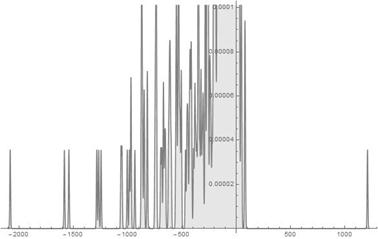
Fig. 1. S-Histogram of experimental 1-dimensional frequency distribution function at t = 236.

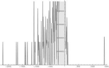
Fig. 2. S-Histogram of experimental 1-dimensional frequency distribution function at t = 242.

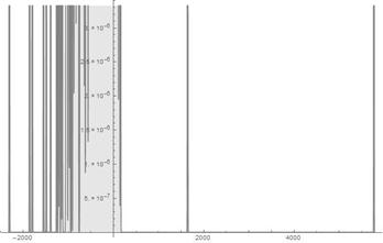
Fig. 3. S-Histogram of experimental 1-dimensional frequency distribution function at t = 248.

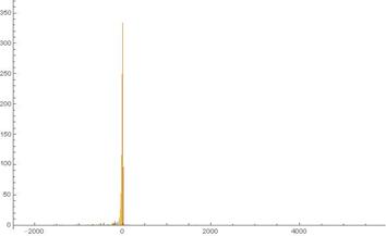
Fig.4. Histogram of experimental 1-dimensional frequency distribution function at t = 248.

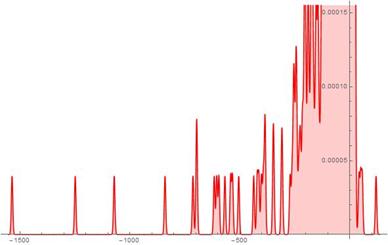
Fig. 5. S-Histogram of experimental 1-dimensional frequency distribution function at t=186.

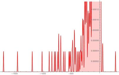
Fig. 6. S-Histogram of experimental 1-dimensional frequency distribution function at t=200.

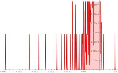
Fig. 7. S-Histogram of experimental 1-dimensional frequency distribution function at t=215.

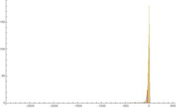
Fig. 8. Histogram of experimental 1-dimensional frequency distribution function at t=215.

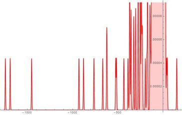
Fig. 9. S-Histogram of experimental 1-dimensional frequency distribution function at t =216.

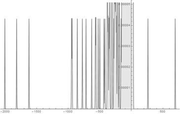
Fig. 10. S-Histogram of experimental 1-dimensional frequency distribution function at t =224.

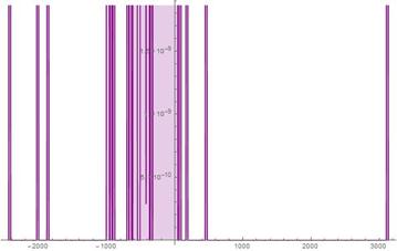
Fig. 11. S-Histogram of experimental 1-dimensional frequency distribution function at t =236.

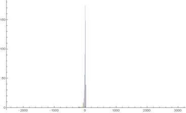
Fig. 12. Histogram of experimental 1-dimensional frequency distribution function at t =236.

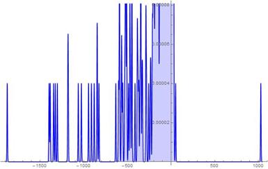
Fig. 13. S-Histogram of experimental 1-dimensional frequency distribution function at t = 212.

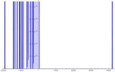
Fig. 14. S-Histogram of experimental 1-dimensional frequency distribution function at t = 213.

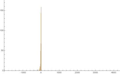
Fig. 15. Histogram of experimental 1-dimensional frequency distribution function at t = 213.

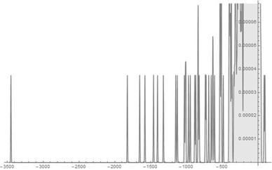
Fig. 16. S-Histogram of experimental 1-dimensional frequency distribution function at t = 220.

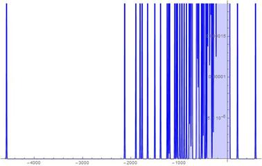
Fig.17. S-Histogram of experimental 1-dimensional frequency distribution function at t = 232.

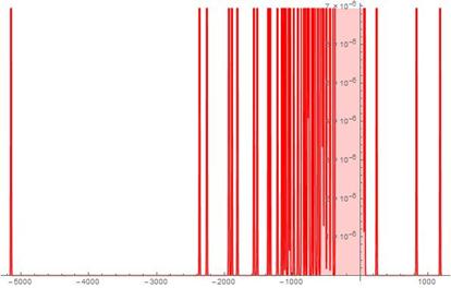
Fig. 18. S-Histogram of experimental 1-dimensional frequency distribution function at t = 238.

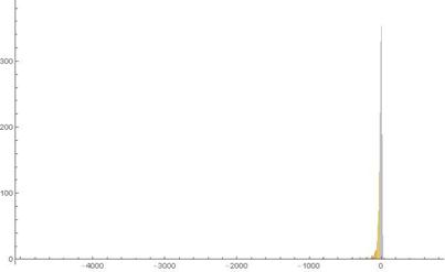
Fig. 19. Histogram of experimental 1-dimensional frequency distribution function at t = 238.

The last two series are devoted to study how much the Brownian walk dynamics of the particles depends on the parameter  whose value is dominant over that of all the other parameters in influence that the vivacity exerts on ability of the particles to penetrate through the high friction barrier. In Ser. 4 and Ser. 5, its value is equal to  and  respectively. These values are more than that are fixed before in two and four times respectively. A principal result of the numerical experiments fulfilled with the given values of consists in continuation of existence of the same Brownian particle walk scenario of that we introduce above with. But a realization of this scenario takes place with the other start points, namely:  in Ser. 4 and  in Ser. 5 while in Ser. 3,  only. What else is worthy to especially notice here is the extremely highest speed which the "tunnelling" particle penetrates though the friction barriers with. So, comparing Figs. 13-14 of Ser. 4, we should pay attention to such the event of interest: for a time while, the "tunnelling" particle runs a distance from  till , i.e. almost instantly in a sense. However questions of whether this phenomenon of the extremely highest speed of displacement and "tunnelling" of the particles is a fundamental feature of the model under study or one is produced by a special dependence choice of on the vivacity  and whether changing of that to, where , can result in disappearance of the given phenomenon remain a matter for further consideration in somewhere else.

As for figures in Ser. 5, they serve to the very important purpose to show that increasing of the parameter values leads to a considerable slowing down of the aforementioned dynamics. Really, observing successively Figs. 16-18 of Ser. 5 and comparing them with the previous series figures we can plain establish that, in the last case, scattering of the particles from the start point runs much slower than in the previous ones. It results in turn in a certain visible stagnation in development of dynamics of the experimental frequency distribution function. In particular, the very same visible stagnation and slowing down one can observe in both the "tunnelling" particles appearance and their movement in depth of the positive axis half too. Summarizing all what is just said above one can make a conclusion that increasing of the value of  towards 0 cannot lead to cancellation of appearance of the "tunnelling" particles penetrating through the high friction barrier although can slow down the Brownian particles walk dynamics development rather than in appearance of the "tunnelling" particles. One more aspect distinguishing Ser. 5 experiments from those of Ser. 1-4 is limits of displacement of the particles along the -axis. Namely: in this series one of the particles runs in the left axis half considerably further then the "tunnelling" particles penetrate in depth of the right axis half.

After these principal sentences, let us say some additional remarks. As we mentioned already increasing of  under keeping of the rest parameter values results, as a rule, in increasing values of  which guarantee the "tunnelling" particle appearance. However, the numerical experiment results under review show that if simultaneously with increasing of  to increaseto the values pointed out above one can observe that the aforesaid phenomenon does not take place then at all. In doing so the aforementioned values of must on the contrary decrease. Besides, we want to notice attention once more on an extreme fewness of the penetrating particles and to stress that their number may be, as it is well-seen from the presented histograms, even 1 or 2. However these few particles penetrate in depth of the positive axis half very quickly and in doing so considerably far off than those particles which penetrate in depth of the negative axis half. A propos a number of latter particles, as it is well-seen from the S-Histograms, is much more than that of the former ones. Nevertheless the Histograms all show that the Brownian walks of the most fraction of particles concentrate nearby their start point.

4. Conclusions

Before to make final conclusions from all what is the aforesaid we should attract readers’ attention to that all the simulations are fulfilled with aid of a notebook. Hence its computational possibilities confined us in making numerical experiments. In particular, 3072 being a number of particles under study and 248 being a time of observation are quantities extremely close to limit for this notebook to make computations described above. Nevertheless it is not able to prevent us to make entirely substantiated conclusions for dynamics of the Brownian walk for sets having more than 3072 particles for times more than 248. Really, it is plain the more particles taking place in the dynamics and the longer time of observation of their dynamics the dynamics the more statistical probability to observe some event or phenomenon. We were convinced in the said above when made series of numerical experiments with the 2048 particles during a while equal to 186 and, in doing so, do not observe the active particle penetration (tunnel effect). After this preface we are ready to formulate principal sentences.

I. Dynamics of the Brownian active particles walk which appears and develops due to the white noise action differs of respective dynamics for the passive ones. A main feature distinguishing distinctly the former from the latter consists in an appearance of a very few particles whose vivacity under the white noise action rises so much that reaches rates which permit for the given particles to overcome the highest friction barriers and to penetrate in domains lying beyond the barriers. In doing so a size of the active particle ability to accumulate the vivacity depends on the size of , the natural internal frequency or, to be more precise, on . Namely: rising of the values of  results, as one can make infer from the numerical experiments, in quick increasing of the active particle vivacity.

II. Existence of such the kind particles defines by a sign rather than absolute value of  entirely. It must be . As for , under condition of keeping the same of all the other parameter values as well as initial data, it influences on time of appearance of the aforementioned particles. In doing so increasing of values of  towards 0 results either in increasing of time that is necessary to spend for observation in order to pick up the appearance of particles which overcome the friction barriers or in necessity to reduce down then the value of .

III. The model under scrutiny allows to realize and to explain how cosmic particles can get the very high energy travelling in the Universe space. Let us assume that the Universe space-time continuum possesses a characteristic (for preventing of ambiguousness, let it be designated bytoo) analogous by its influence on the cosmic particles energy to that the model parameter of exerts on the active particle vivacity. Let us conjecture additionally that this be a function  whose values fluctuate quickly in time near by a visible mean value being equal to 0. Since the visible value 0 is neutral in the sense that it does not influence for energy accumulating by the cosmic particles due to their mutual collisions, the characteristic itself  may happen unobservable. Thus, there appears a necessity to explain the aforesaid phenomenon. The model under study allows to realise as a whole mechanics of how the cosmic particles in process of only their mutual collisions can accumulate such the highest energy that they obtain ability to penetrate throughout energetic barriers.

References

1. Rěvěsz P. Random walk in random and non-random environments. WorldScientific. Singapore, 1990.
2. Haken H. Synergetics. Springer. Berlin, 1983.
3. Haken H. Advanced synergetics. Springer. Berlin, 1985.
4. Zaslavsky G.M., Sagdeev R.Z., Usikov D.A. and Chernikov A.A. Weak chaos andquasi-regular patterns. Cambridge University Press, Cambridge, 1987.
5. Schuster H.G. Deterministic Chaos. Springer. 3^rd edition. Berlin, 1995.
6. Karatzas I. and Shreve S.E. Brownian motion and stochastic calculus, Springer.2^nd edition. Berlin, 1996.
7. Vavrin D.M., Ryabov V.B., Sharapov S.A. and Ito H.M. Chaotic states of weaklyand strongly nonlinear oscillators with quasiperiodic excitation. Phys. Rev E 53,1996, pp. 103-114.
8. Doering Ch.R., Sargsyan Kh.V. and Smereka P. A numerical method for somestochastic differential equations with multiplicative noise. Physics Letter A,vol. 344, 2005, pp. 149-155.
9. Rossler A. Runge-Kutta methods for Ito stochastic differential equations withScaler noise. BIT Numerical Mathematics, vol. 46, 2006, pp. 97-110.
10. Socha L. Linearization methods for stochastic dynamic systems, Springer, Berlin,2008.
11. Archambear C. and Opper M. Approximation influence for continuous-timeMarkov processes. In: Baysesian Time Series Models, chapter 6, pp. 125-140,Cambridge University Press, Cambridge, 2011.
12. Sarkka S. and Sarmavuori J. Gaussian filtering and smoothing for continuous-Discrete dynamic systems. Signal Processing, vol. 93, 2013, 500-510.
13. Ivanov M.A, Dobrynskiy V.A. Random walk of oscillator on the plane withnon-homogeneous friction. Int. INFA-ANS J. Problems Nonlinear Analysis inEngineering Systems", vol. 12, no. 1(15), 2006, pp. 101-116.
14. Ivanov M.A, Dobrynskiy V.A. Stochastic dynamics of oscillator drift in mediawith spatially non-homogeneous friction, J. Automation and Information Sci.,vol. 40., no. 7, 2008, pp. 9-25.
15. Dobrynskii V.A. Unusual frequency distribution function shape generated byparticles making Brownian walk along line with monotone increasing friction,Int. J. of Mathematics and Computation Sci., vol. 1., no. 3, 2015, pp. 91-97.