Calculation of Lagrange Points by Solving Non-linear System Using Taylor Method

Mirzaei Mahmoud AbadiVahid^{1, *}, Askari Mohammad Bagher², Mirhabibi Mohsen²

¹Faculty of Physics, Shahid Bahonar University, Kerman, Iran

²Department of Physics, Payame Noor University, Tehran, Iran

Abstract

After introducing Lagrange points, it is tried to offering three body systems for example sun, earth, and satellite system, two force components equations in orbital plane in center of mass coordinate. Then with formation of a non-linear equations system, the roots of this system by Taylor method are solved. These roots are the roots of force component and in other word are the Lagrange points. Finally, calculated Lagrange points by numerical Taylor method for discussed example are compared with other references.

Keywords

Lagrange Points, Non-linear System, Taylor Method, Earth, Sun, Moon

Received: June 2, 2016
Accepted: October 26, 2016
Published online: November 2, 2016

@ 2016 The Authors. Published by American Institute of Science. This Open Access article is under the CC BY license. http://creativecommons.org/licenses/by/4.0/

1. Introduction

Lagrange points are named in honor of Italian-French mathematician Joseph-Louis Lagrange. [1] There are five special points where a small mass can orbit in a constant pattern with two larger masses. The Lagrange Points are positions where the gravitational pull of two large masses precisely equals the centripetal force required for a small object to move with them. [2] A Lagrange point is a location in space where the combined gravitational forces of two large bodies, such as Earth and the sun or Earth and the moon, equal the centrifugal force felt by a much smaller third body. Lagrangian points are proposed for three-body system in astronomy for example, solar system, the Earth and the satellite. Lagrange points are places where the resultant gravity of the sun and the earth satellite, satellite filed in line with the center of solar masses and the Earth, and the centrifugal force are in balance. [3] Proved that the solar system, terrestrial and satellite, there are five Lagrangian point of the Sun and the Earth filed three points on the line and two other points is XY plane (Earth-Sun orbital plane). In Figure 1 the solar system and the Earth is shown. In this figure, M1 and M2 to the solar masses and the Earth and the origin of the coordinate system the center of mass of the Sun-Earth system are intended. [4] According to the coordinate's vector r, vector towards the center of gravity location, location relative to the sun vector r₁-r vector and the vector r₂-r is the vector location relative to the Earth. Earth-Sun distance as shown in Figure R is intended. [5]

2. Taylor Series

In mathematics, a Taylor series is a representation of a function as an infinite sum of terms that are calculated from the values of the function's derivatives at a single point. The concept of a Taylor series was formulated by the Scottish mathematician James Gregory and formally introduced by the English mathematician Brook Taylor in 1715. [6] If the Taylor series is centered at zero, then that series is also called a Maclaurin series, named after the Scottish mathematician Colin Maclaurin, who made extensive use of this special case of Taylor series in the 18th century. A function can be approximated by using a finite number of terms of its Taylor series. Taylor's theorem gives quantitative estimates on the error introduced by the use of such an approximation. The polynomial formed by taking some initial terms of the Taylor series is called a Taylor polynomial. The Taylor series of a function is the limit of that function's Taylor polynomials as the degree increases, provided that the limit exists. A function may not be equal to its Taylor series, even if its Taylor series converges at every point. A function that is equal to its Taylor series in an open interval is known as an analytic function in that interval. Several methods exist for the calculation of Taylor series of a large number of functions. [7]

One can attempt to use the definition of the Taylor series, though this often requires generalizing the form of the coefficients according to a readily apparent pattern. Alternatively, one can use manipulations such as substitution, multiplication or division, addition or subtraction of standard Taylor series to construct the Taylor series of a function, by virtue of Taylor series being power series. In some cases, one can also derive the Taylor series by repeatedly applying integration by parts. Particularly convenient is the use of computer algebra systems to calculate Taylor series.

The trigonometric Fourier series enables one to express a periodic function (or a function defined on a closed interval [a, b]) as an infinite sum of trigonometric functions (sines and cosines). In this sense, the Fourier series is analogous to Taylor series, since the latter allows one to express a function as an infinite sum of powers. Nevertheless, the two series differ from each other in several relevant issues.

Obviously the finite truncations of the Taylor series of f(x) about the point x = a are all exactly equal to f at a. In contrast, the Fourier series is computed by integrating over an entire interval, so there is generally no such point where all the finite truncations of the series are exact. Indeed, the computation of Taylor series requires the knowledge of the function on an arbitrary small neighbourhood of a point, whereas the computation of the Fourier series requires knowing the function on its whole domain interval. In a certain sense one could say that the Taylor series is "local" and the Fourier series is "global."

The Taylor series is defined for a function which has infinitely many derivatives at a single point, whereas the Fourier series is defined for any integrable function. In particular, the function could be nowhere differentiable. (For example, f(x) could be a Weierstrass function.) [8]

The convergence of both series has very different properties. Even if the Taylor series has positive convergence radius, the resulting series may not coincide with the function; but if the function is analytic then the series converges pointwise to the function, and uniformly on every compact subset of the convergence interval. Concerning the Fourier series, if the function is square-integrable then the series converges in quadratic mean, but additional requirements are needed to ensure the pointwise or uniform convergence (for instance, if the function is periodic and of class C₁ then the convergence is uniform).

Finally, in practice one wants to approximate the function with a finite number of terms, let's say with a Taylor polynomial or a partial sum of the trigonometric series, respectively. In the case of the Taylor series the error is very small in a neighbourhood of the point where it is computed, while it may be very large at a distant point. In the case of the Fourier series the error is distributed along the domain of the function.

3. Calculation of Lagrange Points by Solving Non-linear System Using Taylor Method

Lagrange point is a point of equilibrium binding force on the third body in the Earth-Sun system. Force balance to the third body by the forces of gravity and the force of the sun and the earth rotating around the center of mass of the third body (Sun-Earth) This condition leads to the equation 1:

           (1)

That

                           (2)

r is the vector Lagrangian point location relative to the center of mass of the Sun and Earth [9]. Last sentence in equation (1), a provider of mrω² force on the third body. It is assumed that ω is constant for all Lagrangian points.

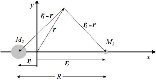
Fig. 1. Sun-Earth system's in the center of mass coordinate system.

Balance of forces leading to the equations 3 and 4.

                   (3)

               (4)

To determine if there is enough sun and Earth Lagrange point on the line is filed in equations (3) and (4) the value of y will be zero. If the two equations (3) and (4) the value of y is zero-equation 5 and 6 are obtained.

                  (5)

                               (6)

The condition y = 0 (on axis x) function g (x, y) is always zero. So just need to follow the x-axis zeros of the function f (x, y = 0), the equation (5). To find the roots of a univariate function f (x, y = 0), can be used conventional methods. But we must be careful, there are a singular point of f (x, y = 0). Singularities corresponding to the location of the center of mass of the Sun and the Earth. Function is plotted in Figure 2. This curve is the approximate location of the specified root.

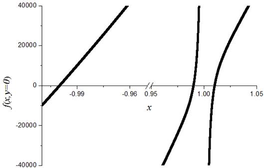
Fig. 2. Curve f (x, y = 0), the figure is the approximate location of the roots.

Assuming the Earth to the Sun, ^6-10×3, and the distance from the Sun to Earth 1Au, Filed Earth-Sun Lagrangian points on the line (y = 0) is achieved. By chord root method x₁= 1.000001-and x2=0.990016 and x₃=1/ 010045 achieved accuracy by 10^-6. The Earth and the Sun Lagrangian points, respectively filed on line 1. 000 001, 0.990016 and 1.010045 times the distance Earth-Sun is the center of mass of the source device. Negative roots based on the coordinate system shown in Figure 1 on the opposite side of the earth relative to the sun. To calculate the Sun-Earth Lagrange point which matches the lines are not filed the Taylor method can be used to solve the equations. The method for solving equations is as follows:

                                (7)

With an initial estimate of solutions (x₀, y₀) is as follows:

                         (8)

In this equation

                   (9)

And

         (10)

Programs written in FORTRAN, by Taylor method. The numerical solution obtained has a good agreement with similar calculation. The answer includes:[10]

(0.866025- ،0.499997) and (0.866025 ،0.499997)

4. Result and Discussion

All the Lagrangian points can be obtained by introducing a coordinate system that actually components of a category equation resultant force acting on the satellites in Sun-Earth. In the majority of calculations per point Lagrange equation has been introduced that gives the roots of the equation Lagrange point. In other words, given an equation for each Lagrange point. It means that for five Lagrangian points can be written five equations. The function f (x, y) and g (x, y) to power components as they the singularities. These points make it difficult to find the roots of the two functions simultaneously. Results from programs written answer with the same things show good agreement it confirms the accuracy of the method is employed.

References

1. Pluchino, Salvatore, Nicolo Antonietti, and Claudio Maccone. "Protecting the Moon farside radio-telescopes from RFI produced at the future Lagrangian-Points space stations." Journal of the British Interplanetary Society 60.5 (2007): 162-168.
2. Boss, Alan P. "Giant planet formation by gravitational instability." Science 276.5320 (1997): 1836-1839.
3. Heisenberg, Werner. The physical principles of the quantum theory. Courier Corporation, 2013.
4. Koon, Wang Sang, et al. "Dynamical systems, the three-body problem and space mission design." Free online Copy: Marsden Books (2008).
5. arlson, Andrew. "The Logisitics Development of a cis-Lunar Transfer Vehicle." AIAA SPACE 2011 Conference & Exposition. 2011.
6. Dehn, Max, and E. D. Hellinger. "Certain mathematical achievements of James Gregory." The American Mathematical Monthly 50.3 (1943): 149-163.
7. Warming, R. F., and B. J. Hyett. "The modified equation approach to the stability and accuracy analysis of finite-difference methods." Journal of computational physics 14.2 (1974): 159-179.
8. Runge, Erich, and Eberhard KU Gross. "Density-functional theory for time-dependent systems." Physical Review Letters 52.12 (1984): 997.
9. Seidov, Zakir F. "The Roche problem: some analytics." arXiv preprint astro-ph/0311272 (2003).
10. Henrard, Jacques. "The web of periodic orbits at L 4." Celestial Mechanics and Dynamical Astronomy 83.1-4 (2002): 291-302.