
International Journal of Energy and Sustainable Development, Vol. 1, No. 1, December 2016 Publish Date: Aug. 19, 2016 Pages: 6-12
Review of Existing Models for Stirling Engine Performance Prediction and the Paradox Phenomenon of the Classical Schmidt Isothermal Model
Kwasi-Effah C. C.1, *, Obanor A. I.1, Aisien F. A.2, Ogbeide O.3
1Department of Mechanical Engineering, University of Benin, Benin City, Nigeria
2Department of Chemical Engineering, University of Benin, Benin City, Nigeria
3Department of Production Engineering, University of Benin, Benin City, Nigeria
Abstract
The Schmidt model is one of the classical methods used for developing Stirling engines. The Schmidt analysis is based on the isothermal expansion and compression of an ideal gas. However with the recent innovation in technology, the Schmidt analysis needs to be improved upon as this analysis has been found to include phenomenon which contradicts the real behavior of the Stirling engine. In this paper the Schmidt analysis used in the performance prediction of the gamma-type Stirling engine is derived and lapses in this model is identified orderly. Other popular models developed by various individuals including their assumptions and limitations are described in this paper.
Keywords
Stirling Engine, Thermodynamic Model, Schmidt Analysis, Performance Prediction
Received:July 18, 2016
Accepted: August 3, 2016
Published online: August 19, 2016
@ 2016 The Authors. Published by American Institute of Science. This Open Access article is under the CC BY license. http://creativecommons.org/licenses/by/4.0/
Contents
1. Introduction
During the 1950’s, a number of studies were performed to develop empirical correlations for estimating the Stirling engine performance parameters based on power output and the engine efficiency [1]. The Beale number as described by Koichi in 1998 is a common method used to empirically predict or estimate the power output of the Stirling engine [2]. Professor William Beale, of Sunpower Inc. in Athens, Ohio, conformed that the power output of many Stirling engines can be approximated by Equation (1).
P = Be *Pmb* f* Vob (1)
This can be rearranged as:
Be = ![]() = constant (2)
= constant (2)
The equation was found by Beale to apply roughly to various kinds and sizes of Stirling engines for which information were accessible including free piston machines and those with kinematic linkages. In many cases, the engines operated with heater temperature gradient ranging between 65°C and 650°C. Figure 1 shows the plot of Beale number versus heater temperature. The result of Equation (2) is a dimensionless group which is known as the Beale number. In Martini's report, another strategy exists to estimate the performance of a Stirling engine, in support to Beale's equation. The equation utilizes the process temperatures [1]. This method was found by West and is given by:
P = F.n.Pmw.Vo. ![]() (3)
(3)
Where,
F = 0.35 (West factor)
Figure 1. Beale number as a function of the heater temperature.
Source: [1]
In order to find an appropriate correlation for calculating the power output of the Stirling engine precisely that of the gamma configuration, Kongtragool, and Wongwises in 2003 investigated the experimental performance of a gamma type Stirling engine [3]. They came to the conclusion that the Beale’s formula was not valid for conditions in which there were high-temperature ratio. However, they recommended that the original Beale formula and the mean pressure based power output formula with a certain magnitude of the factor F (0.25 – 0.35) representing mechanical loss and friction coefficient would make it possible to accurately predict the engine’s power output. The mean pressure equation is similar to the West equation given as follows:
P = Fopmw fVp![]() (4)
(4)
In order to improve further, the empirical correlations for predicting the Stirling engine performance, [4] analysed a wide range of experimental results and applied methods of the dynamic similarity and quasi-static simulations for various types of Stirling engines. They used dimensionless analysis to characterize the gas leakage and mechanical power losses present in an actual Stirling engine. The dimensionless mechanical power losses were determined using the empirical data. Several Stirling engines were modeled. Prieto et al. found that such correlation based on dimensionless analysis of the engine’s working process and different losses in the cycle provided more accurate prediction of the performance of the Stirling engines. Empirical models provide a quick way to estimate the relationship between the overall size of an engine and its power output, but they are not very useful as detailed design tools for Stirling engines [5].
The Schmidt isothermal model was published in 1871 by Professor Gustav Schmidt of the German Polytechnic Institute [2]. The Schmidt analysis is a pure mass balance for the working gas of the Stirling engine. It is based upon the theory of an isothermal expansion and compression of an ideal gas. This method allows using some simplifications to calculate the pressure distribution as a function of the crank angle as well as the determination of the cycle work. An advantage of this analysis is that the equation set can be solved in a closed form and so there is no need to use numerical procedures. The limiting factor of this model is that most assumptions are based on ideal condition; the only non-ideal condition is the assumption of sinusoidal continuous variation of the piston movement as against the discrete movement of the ideal cycle. [6] Presented a model which takes into account the effectiveness of the drive mechanism in the Schmidt theory to analyze the engine performance of the gamma type configuration. The results of experiments on a 10 kW gamma type Stirling engine demonstrated that the mechanical effectiveness of the engine has a strong influence on the shaft power of engine. Martini presented an isothermal model based on Schmidt theory and taking into account heat losses and pressure losses. The temperatures of hot and cold gases were obtained by taking into account temperature drops in the heater and cooler. His model was validated using the experimental data obtained from GPU-3 Stirling engine. There was 20% error compared to experimental results [7]. Finkelstain developed an adiabatic analysis. His model defined an adiabatic compression and expansion spaces whilst all heat exchangers were treated as perfect heat exchangers with isothermal [8]. As reported by [9], Qvale developed a model for predicting the heat input, work output, and indicated efficiency of a Beta type Stirling engine based on adiabatic and sinusoidal conditions. Results of his model compared favorably with the test data over a range of engine speed (1500 to 3000 rpm). Rio devised a model by developing further Qvole's work on the adiabatic second-order model. Rio used the same basic assumptions as Qvole but changed the formulation of the problem so that nonsinusoidal piston displacements could be specified. Rio’s model was typically based on Stirling refrigeration. Lee Allan developed an adiabatic analysis in 1973, which provides a unique power loss mechanism which involves the cyclic heat transfer loss. Model by [10] involved an adiabatic and isothermal analysis with objectives in low temperature ratio applications; Shoureshi developed two Stirling engine mathematical models. The complete model was an improvement of Rio’s adiabatic model. For mechanical friction loss, Shoureshi developed a correlation based on internal combustion engine data. In 1977, Urieli in an attempt to establish basic trends, presented a simplified closed form analysis based on idealized cycles but without the mechanical or thermodynamic restriction imposed by Schmidt on the alpha type Stirling engine [11]. In particular he examined the effect of non isothermal compression and expansion. The major assumption made was that all particles of working fluid undergo the same process throughout the cycle. The result of his analysis showed that it is possible to operate the ideal Stirling cycles at high volume compression ratio for high power output and efficiency however, it seemed detrimental to operate the non-ideal Stirling at high volume compression ratio. In 1983, Roy and Tew developed a model which was referred to as the common pressure analysis. They used the conservation of mass, energy, and equation of state to determine the thermodynamics of the gas at each node. Several simplifications were used to minimize the numerical integration. The momentum equation was totally ignored and a common pressure through each gas nodes was assumed during each time step. Roy and Tew compared their model with experimental data from the GPU-3 Stirling engine. When the regenerator friction factor was increased by factors of 4.0 and 2.6 for hydrogen and helium, respectively, the model over predicted both brake power and efficiency by 5 t o 30% [12].
2. Derivation of the Schmidt Model for Gamma Type Stirling Engine
In the Schmidt model, the gamma types Stirling engine is considered as having five control volumes serially connected together as appeared in Figure 2. This comprises of a compression space c, expansion space e, heater h, cooler k, and regenerator r. Every cell is considered as a homogeneous element, the gas is represented by its instantaneous mass m, volume V, absolute temperature T and pressure P with suffix c, k, r, h, and e representing the particular cell.
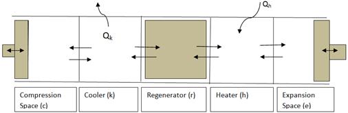
Figure 2. Control volumes of the ideal Isothermal model.
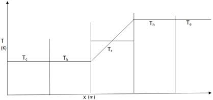
Figure 3. Temperature profile of the ideal isothermal model.
The condition made in this analysis is that the gas in the expansion space and the heater is at constant upper source temperature and gas in compression space and the cooler is at constant lower temperature. Hence the isothermal condition assumed makes it conceivable to generate a basic expression for the working fluid pressure as a function of the volume variations. To get closed form solution, Schmidt accepted that the volumes of the working spaces fluctuate sinusoidally. The assumed isothermal condition of the working spaces and heat exchangers suggests that the heat exchangers including the regenerator are very effective. The beginning stage of the analysis is that the total mass of gas in the engine is constant as follows:
M = mc + mk + mr + mh + me (5)
Substituting the ideal gas law given by Equation (6)
m = ![]() (6)
(6)
We obtain
![]() = MR (7)
= MR (7)
With specific end goal to evaluate the total mass of gas in the void space of the regenerator, the lengthwise distribution of the working fluid temperature must be known. [11] demonstrated that for real regenerators, the temperature profile is linear, and consequently, it was expected that the ideal regenerator has a temperature profile which is linear between the hot temperature and cold temperature, as shown in Figure 4.
The assumption of a linear temperature profile can be numerically defined by the equation of a straight line as follows:
T(x) = ![]() + Tk (8)
+ Tk (8)
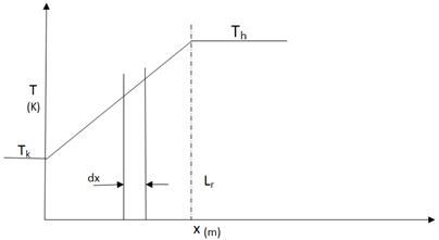
Figure 4. Regenerator linear temperature profile.
The summation of mass of gas contained in the void volume of the regenerator, is obtained by
mr = ![]() (9)
(9)
Where 𝝆 is the density,
dVr, = Ardx (10)
Where dx is the derivative volume for constant free flow area A, and Vr = ArLr.
Where Ar can be written as:
Ar=![]() (11)
(11)
Substituting (10), (11) and the ideal gas law p = 𝝆 RT in Equation (9) thus:
mr = ![]() dx (12)
dx (12)
Integrating Equation (12) and simplifying:
mr = ![]() (13)
(13)
Defining the effective mean temperature (T) of the regenerator, in terms of the ideal gas equation of state:
mr = ![]() (14)
(14)
Next, comparing Equations (13) and (14) we obtain:
Tr =![]() (15)
(15)
Given the volume variations Vc and Ve we can evaluate Equation (13) for pressure as being a function of the volume variation of the expansion and compression space.
P =  (16)
(16)
The work done by the Stirling engine for a single cycle can be obtained by the cyclic integral of pdV
W = We + Wc = ![]() (17)
(17)
Considering the energy equation of the ideal isothermal model from the perspective of energy flow, the transfer of heat into and out of the system occurs at the cold and hot temperatures Tk and Th. Enthalpy is transported into the cell by method for mass flow mi and temperature Ti, and out of the cell by method for mass flow mo and temperature To as shown in Figure 5.
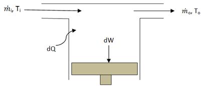
Figure 5. Generalized cell of energy flow.
The statement of the energy equation for the working gas in the generalized cell is as follows:
We know that:
Specific enthalpy hs = cp T (18)
Specific internal energy us = cv T (19)
Where cp and cv are the Specific heat capacities of the working fluid (gas) at constant volume and pressure.
Therefore substituting in Equation (18) we have:
dQ + (cp Ti mi - cp To mo) = dW + cv d(m T) (20)
Equation (21) is the non-steady flow energy equation in which kinetic and potential energy terms have been ignored. In the Schmidt isothermal model for the compression and expansion spaces, and additionally for the cooler and heater, we have T= Ti = To, a constant value. Moreover, from mass conservation equation, the difference in the mass flow (![]() i-
i- ![]() o) is equal to the rate of the mass amassing inside of the cell dm. Equation (20) along these lines simplifies to:
o) is equal to the rate of the mass amassing inside of the cell dm. Equation (20) along these lines simplifies to:
dQ + cp d(Tm) = dW + cv d(Tm) (21)
dQ = dW – Rd(Tm) (22)
For the assumed ideal gas, the gas constant (R) is given by:
R = cp - cv (23)
Hence,
cp =R![]() (24)
(24)
cv = R![]() (25)
(25)
With
λ = ![]() (26)
(26)
Qc = Wc, Qe = We (27)
So also, for the heat exchanger spaces, since work done is zero we have:
Qk = 0, Qh = 0, Qr = 0 (28)
Hence, the cycle efficiency can be given accordingly by:
η=![]() (29)
(29)
For the ideal regenerator Qr = 0. This is due to the fact that the heat exchange between the regenerator and the working fluid is internal. There is no transfer of heat externally between the regenerator and the open environment.
In order to unravel these equation sets, the working space volume variations Vc and Ve and the derivates dVc and dVe with respect to crank angle θ needs to be known.
To solve the differential equation set, Schmidt made an assumption of a sinusoidal variation in the expansion and compression space as over a solitary cycle.
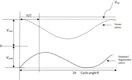
Figure 6. Sinusoidal volume variation of compression and expansion space of the gamma type Stirling engine.
Vc = Vclc + ![]() +
+ ![]() (30)
(30)
Ve = Vcle + ![]() (31)
(31)
Substituting for Vc and Ve in Equation (25) and simplifying we have:
 (32)
(32)
P=![]() (33)
(33)
P=![]() (34)
(34)
P=![]() (35)
(35)
Where
s = ![]() (36)
(36)
Given:
Acos![]() + Bcos(
+ Bcos(![]() ) = Ccos(
) = Ccos(![]() ) (37)
) (37)
Where
β=tan-1 ![]() (38)
(38)
And
C= ![]() (39)
(39)
By utilize the trigonometric substitution of β and c, we can simplify Equation (37) as follows:
β=tan-1  (40)
(40)
C= ![]() (41)
(41)
Therefore,
P = ![]() (42)
(42)
Hence we obtain:
P = ![]() (43)
(43)
Pmin = ![]() (44)
(44)
Pmax = ![]() (45)
(45)
Pmean =![]() (46)
(46)
Pmean = ![]() (47)
(47)
Pmean = ![]() (48)
(48)
![]() =
= ![]() (49)
(49)
![]() =
= ![]() -
- ![]() (50)
(50)
W = ![]() +
+ ![]() (51)
(51)
3. Discussions
Several mathematical models exist to predict the performance characteristics of the Stirling engine based on various assumptions. These models can assist in the improvement of the Stirling engine performance. However, there are varying degrees of errors in all these models. Thus, the degree of accuracy of a model is a function of the realistic assumptions made and number of parameters taken into consideration.
Equation (51) defines a relationship to obtain the work done of a gamma type Stirling engine configuration. By taking a close look at the Equation (27) to (28) we observe that all the heat exchangers in the ideal Stirling engine are not functioning and external heat transfer happens across the boundaries of the compression space Qc and expansion spaces Qe. The implication of this is that the work done in the compression and expansion space is a contributory factor of only the heat energy Qe and Qc without any external support from the heat exchangers. This can be confusing in actual sense since Qe and Qc cannot generate their own energy independent of the heat exchangers Qh and Qk. This unmistakable inconsistency is an immediate result of the definition of the Ideal Isothermal analysis where the expansion and compression spaces are maintained at the heater and cooler heat exchangers temperatures. In real engines, the compression and expansion spaces will have a tendency to be adiabatic as opposed to isothermal, which infers that the net heat transferred over the cycle must be given by the heat exchangers.
4. Conclusion
Reviews on various numerical and empirical models have been discussed. The prevalent Schmidt thermodynamic model was derived and constraining factors in this model were made known. In the Schmidt analysis, the compression and expansion spaces were kept up at the specific heater and cooler heat exchanger temperatures. This prompted the confusing circumstance that neither the cooler nor the heater contributed any net heat transfer over the cycle and subsequently were redundant. Based on the Schmidt model, the heating energy needed for the system to run happened across the boundaries or limit of the isothermal working spaces (i.e compression and expansion space). Clearly this can't be valid in real systems. In real engines, the working spaces will have a tendency to be adiabatic instead of isothermal, which infers that the net heat transferred over the cycle must be given by the heat exchangers. In this way, it will be more realistic to consider an adiabatic condition for the system boundary and further account for losses in the real system.
References
- Martini, W.R., (1983): Stirling engine design manual. Second edition. 1 NASA CR-168088: 79–80.
- Koichi, H.,(1998): Performance prediction method for Stirling Engine. Available at www.nmri.go.jp/eng/khirata/stirling/pdf.
- Kongtragool, B. and Wongwises, S. A., (2003): Review of solar powered Stirling engines and low temperature differential Stirling engines. Renewable and Sustainable Energy Reviews, Vol. 7: 131–54.
- Prieto, J.I and Stefanovskiy, A.B., (2003). Dimensional analysis of leakage and mechanical power losses of kinematic Stirling engines. Journal of Mechanical Engineering and Science. Vol. 217: 21-36.
- Smith, A.G. and Newman, W., (2012). Analysis of hybrid fuel-cell/stirling-engine systems for domestic combined heat and power. Energy tech Vol.1: 1–7.
- Toda, F. S., Iwamoto, K. and Nagajima, N., (2007). Development of low-temperature difference Stirling engine behavior of the mechanism effectiveness for the performance prediction method. Proceeding of 13th International Stirling engine Conference, Tokyo.
- Chen, N.C. and Griffin, F.P., (1983). A review of Stirling engine mathematical models. Report No ORNL/CON 135, OAK Ridge National Laboratory, Tennessee.
- Martinez, S., (1994). Some mathematical models to describe the dynamic behavior of the B-10 free-piston Stirling engine. Technical report. Russ College of Engineering, Ohio USA.
- Malroy, E. T., (1998). Stirling model with coupled first order differential equations by the Pasic method. Technical report. Ohio University, USA.
- Shoureshi, R., (1982). Analysis and design of Stirling engine for waste heat recovery. PhD Thesis, Massachusetts institute of technology (MIT) USA.
- Urieli, I., (1977). Simulation of Stirling cycle machines. PhD Thesis, Witwatersrand Johannesburg, South Africa.
- Roy, C. and Tew, J.R., (1983). Computer program for Stirling engine performance calculations. DOE/NASA/51 040-42 NASA TM-82960. Available at http://ntrs.nasa.gov/archive/nasa/casi.ntrs.nasa.gov/19830009152.


