Financial Risk Management in Portfolio Optimization with Lower Partial Moment

Lam Weng Siew^{1, 2, *}, Lam Weng Hoe^{1, 2}

1Department of Physical and Mathematical Science, Faculty of Science, Universiti Tunku Abdul Rahman, Kampar Campus, Kampar, Perak, Malaysia

²Centre for Mathematical Sciences, Centre for Business and Management, Universiti Tunku Abdul Rahman, Kampar Campus, Kampar, Perak, Malaysia

Abstract

The mean-lower partial moment model has been proposed in portfolio optimization to minimize the portfolio risk. This model employs mean as the return measure and lower partial moment as the risk measure. Lower partial moment is a downside risk measure in portfolio optimization. The investors will be able to minimize the portfolio risk in their investment by using the mean-lower partial moment model. The objective of this paper is to construct the optimal portfolio using the mean-lower partial moment model with the degree set as 1, 2 and 3. The data of this study comprises weekly return of 20 component stocks of FTSE Bursa Malaysia Kuala Lumpur Composite Index (FBMKLCI) in Malaysia stock market. In particular, the results of this study show that MAXIS is the largest component stock in the optimal portfolio of the mean-lower partial moment model with degree 1, 2 and 3. Besides that, the optimal portfolio of the mean-lower partial moment model with degree 2 gives the portfolio mean return at 0.0010 and portfolio risk at 0.0001. This study is significant because the investor can achieve the target rate of return with minimum portfolio risk.

Keywords

Mean Return, Risk, Semi Variance, Optimal Portfolio, Portfolio Performance

Received:July 17, 2016
Accepted: August 4, 2016
Published online: September 3, 2016

@ 2016 The Authors. Published by American Institute of Science. This Open Access article is under the CC BY license. http://creativecommons.org/licenses/by/4.0/

1. Introduction

Portfolio optimization is an investment strategy in asset selection and allocation [1]. Portfolio optimization is a mathematical approach in making investment decisions of various assets to be included in the portfolio. Portfolio is a grouping of financial assets such as stocks that are held by the investors [2]. Investors desire to achieve the target rate of return at the minimum portfolio risk. Fishburn [3] has introduced the mean-lower partial moment model in portfolio optimization. The mean-lower partial moment model is a mathematical model in portfolio optimization that used to minimize the portfolio risk and can achieve the investors target rate of return. The portfolio risk is represented by the lower partial moment. The lower partial moment is the downside risk that defines risk in terms of probability-weighted functions of deviations below the target return. The mean-lower partial moment model has been studied by the past researchers in portfolio optimization [4-9]. The lower partial moment also has been used as risk measure in handling system design [10]. The objective of this paper is to construct the optimal portfolio using the mean-lower partial moment model based on the components from FTSE Bursa Malaysia Kuala Lumpur Composite Index (FBMKLCI) in Malaysia stock market. The rest of the paper is organized as follow. The next section describes the materials and methods employed in this study. Section 3 discusses about the empirical results of this study. Section 4 concludes the paper.

2. Materials and Methods

2.1. Data

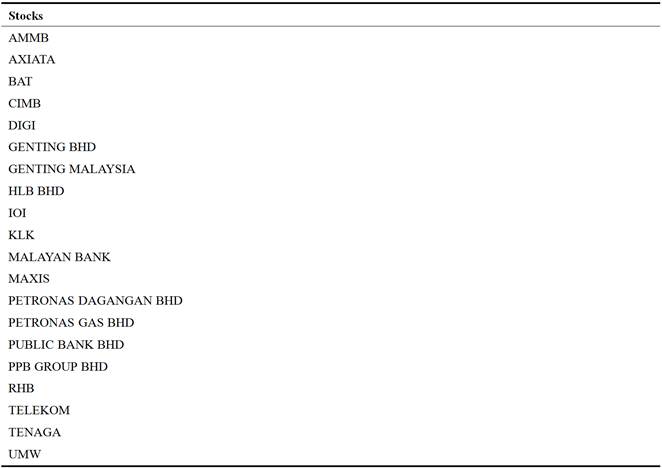
The data of this study comprises weekly return of 20 component stocks of FTSE Bursa Malaysia Kuala Lumpur Composite Index (FBMKLCI) in Malaysia stock market. FBMKLCI is the main indicator of economy in Malaysia. The period of this study covers from November 2009 until December 2014. Table 1 shows the component stocks of FBMKLCI in Malaysia stock market.

Table 1. Component Stocks of FBMKLCI in Malaysia Stock Market.

An optimal portfolio is constructed by using the mean-lower partial moment model. The optimal portfolio composition for each stock will be generated. The summary statistics of the optimal portfolio will also be calculated.

The return of the stocks is determined as below [11].

                               (1)

 is the return of stock i at time t,

 is the closing price of stock i at time t

 is the closing price of stock i at time t-1.

The mean return of the stock i is calculated as below [12].

                                    (2)

 is the mean return of stock i,

 is the return of stock i at time t,

T is the number of observations

Figure 1 shows the construction process of the optimal portfolio with mean lower partial moment model.

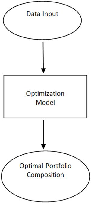
Figure 1. Construction Process of the Optimal Portfolio with Mean Lower Partial Moment Model.

Based on the determination of the optimal portfolio composition using the lower partial moment model, the mean return of the optimal portfolio is formulated as follow [13].

                             (3)

 is the mean return of the optimal portfolio,

 is the mean return of stock i,

 is the amount of the fund invested in stock i,

n is the number of stocks.

2.2. Mean-Lower Partial Moment Model

Fishburn [3] has defined the lower partial moment of order α around  as follows:

=(4)

 is the cumulative distribution function of the investment return ,

 is the benchmark return,

α is the order or degree of the lower partial moment

The mathematical model of mean-lower partial moment model [3] is formulated as follows:

Minimize            (5)

Subject to

                                (6)

                                       (7)

                                          (8)

T is the number of periods,

 is the return of the optimal portfolio at time t,

 is the return of stock i,

 is the weight of each stock in the optimal portfolio,

N is the total number of stocks,

 is the target rate of return.

Equation (5) is the objective function of the model which minimizes the portfolio lower partial moment. Constraint (6) indicates that the portfolio mean return equals to the investors expected rate of return. Constraint (7) indicates that the total weights of all stocks in the optimal portfolio are one. Constraint (8) indicates that the weight of each stock in the optimal portfolio is positive. and α will be set as the expected return and 2 respectively in this study. Besides that, the optimal portfolio of mean-lower partial moment will also be generated in this study with the degree α set as 1 and 3.

Setting α as 2 and  as the expected return will produce the mean-semi variance model. The mean-semi variance model is formulated as follows:

Minimize   (9)

Subject to

                              (10)

                                      (11)

                                     (12)

T is the number of periods,

is the expected return,

 is the return of the optimal portfolio at time t,

 is the return of stock i,

 is the weight of each stock in the optimal portfolio,

N is the total number of stocks,

 is the target rate of return.

Equation (9) is the objective function of the model which minimizes the portfolio semi variance subject to the constraints (10)-(12).

The mean-lower partial moment model has been used to overcome the disadvantage of Markowitz [14] mean-variance model. Markowitz [14] was the pioneer of portfolio optimization by introducing the mean-variance model. Variance is used as risk measure while the mean return is used as the expected return in the mean-variance model. The objective function of the mean-variance model is to minimize the portfolio variance which is the portfolio risk. The lower partial moment is the more appropriate risk measure because the mean-variance model will not only penalize the downside deviation but also the upside deviation which is desirable for the investors.

3. Empirical Results

Table 2 presents the optimal portfolio composition of the mean-lower partial moment model with the degree α set as 1(MLPM1), 2 (MLPM2) and 3 (MLPM3) in percentage.

Table 2. Optimal Portfolio Composition (%).

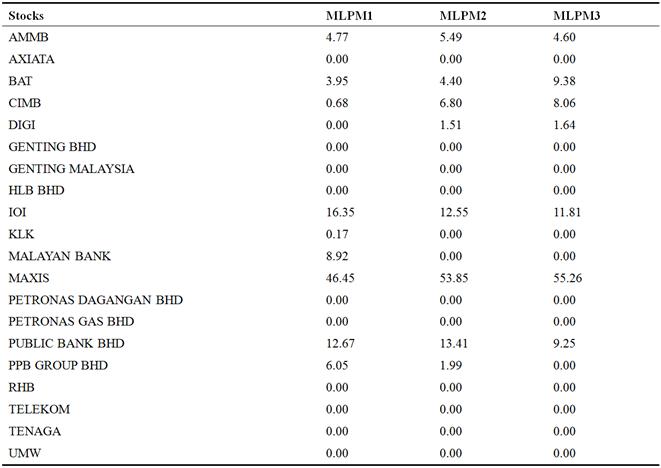
Based on Table 2, the optimal portfolio of the mean-lower partial moment model with degree 1 consists of AMMB (4.77%), BAT (3.95%), CIMB (0.68%), IOI (16.35%), KLK (0.17%), MALAYAN BANK (8.92%), MAXIS (46.45%), PUBLIC BANK BHD (12.67%) and PPB GROUP BHD (6.05%). AXIATA, DIGI, GENTING BHD, GENTING MALAYSIA, HLB BHD, PETRONAS DAGANGAN BHD, PETRONAS GAS BHD, RHB, TELEKOM, TENAGA and UMW are not selected to be included in the optimal portfolio of the mean-lower partial moment model with degree 1 because these stocks give the value 0.00%. MAXIS is the largest component stock because it comprises 46.45% in the optimal portfolio. In constrast, CIMB is the smallest component stock in the optimal portfolio of mean-lower partial moment model with the smallest percentage at 0.68%.

Moreover, the optimal portfolio of the mean-lower partial moment model with degree 2 consists of AMMB (5.49%), BAT (4.40%), CIMB (6.80%), DIGI (1.51%), IOI (12.55%), MAXIS (53.85%), PUBLIC BANK BHD (13.41%) and PPB GROUP BHD (1.99%). AXIATA, GENTING BHD, GENTING MALAYSIA, HLB BHD, KLK, MALAYAN BANK, PETRONAS DAGANGAN BHD, PETRONAS GAS BHD, RHB, TELEKOM, TENAGA and UMW are not selected to be included in the optimal portfolio of the mean-lower partial moment model with degree 2 because these stocks give the value 0.00%. MAXIS is the largest component stock because it comprises 53.85% in the optimal portfolio. On the other hand, DIGI is the smallest component stock in the optimal portfolio of mean-lower partial moment model with the smallest percentage at 1.51%.

In addition, the optimal portfolio of the mean-lower partial moment model with degree 3 consists of AMMB (4.60%), BAT (9.38%), CIMB (8.06%), DIGI (1.64%), IOI (11.81%), MAXIS (55.26%) and PUBLIC BANK BHD (9.25%). AXIATA, GENTING BHD, GENTING MALAYSIA, HLB BHD, KLK, MALAYAN BANK, PETRONAS DAGANGAN BHD, PETRONAS GAS BHD, PPB GROUP BHD, RHB, TELEKOM, TENAGA and UMW are not selected to be included in the optimal portfolio of the mean-lower partial moment model with degree 3 because these stocks give the value 0.00%. MAXIS is the largest component stock because it comprises 55.26% in the optimal portfolio. In constrast, DIGI is the smallest component stock in the optimal portfolio of mean-lower partial moment model with the smallest percentage at 1.64%.

These results indicate that different degree of the mean-lower partial moment model will give different optimal portfolio composition.

Table 3 presents the summary statistics for the optimal portfolio of the mean-lower partial moment model with the degree α set as 1, 2 and 3.

Table 3. Summary Statistics for the Optimal Portfolio Performance of the Mean-Lower Partial Moment Model.

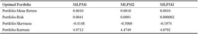
As reported in Table 3, the optimal portfolio of the mean-lower partial moment model with degree 1 gives the portfolio mean return at 0.0010 and portfolio risk at 0.0041. The optimal portfolio skewness as well as kurtosis value is -0.4148 and 4.9712 respectively.

Besides that, the optimal portfolio of the mean-lower partial moment model with degree 2 gives the portfolio mean return at 0.0010 and portfolio risk at 0.0001. This implies that the investors can achieve the portfolio mean return at 0.0010 with the minimum risk of 0.0001. The optimal portfolio skewness as well as kurtosis value is -0.3000 and 4.4749 respectively.

Furthermore, the optimal portfolio of the mean-lower partial moment model with degree 3 gives the portfolio mean return at 0.0010 and portfolio risk at 0.000002. The optimal portfolio skewness as well as kurtosis value is -0.1974 and 4.0792 respectively.

These results indicate that different degree of the mean-lower partial moment model will also give different optimal portfolio risk, portfolio skewness and portfolio kurtosis.

Figure 2, 3 and 4 display the histogram for the optimal portfolio return distribution of the mean-lower partial moment model.

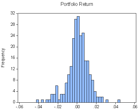
Figure 2. Histogram for the Optimal Portfolio Return Distribution of the Mean-Lower Partial Moment Model with Degree 1.

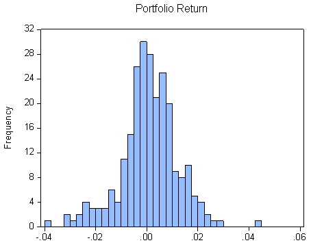
Figure 3. Histogram for the Optimal Portfolio Return Distribution of the Mean-Lower Partial Moment Model with Degree 2.

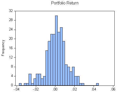
Figure 4. Histogram for the Optimal Portfolio Return Distribution of the Mean-Lower Partial Moment Model with Degree 3.

As displayed in Figure 2, 3 and 4, the distribution of the portfolio return of the mean-lower partial moment model shows positive and negative return. Besides that, the distribution for the optimal portfolio return of the mean-lower partial moment model exhibits skewness.

4. Conclusion

This paper discusses the application of the mean-lower partial moment model in Malaysia stock market. The mean-lower partial moment model is the portfolio optimization model that applied to minimize the portfolio risk. The portfolio risk is represented by the lower partial moment. The optimal portfolio is constructed by using the mean-lower partial moment model with the degree set as 1, 2 and 3 in this study. The results of this study show that different degree of the mean-lower partial moment model will give different optimal portfolio composition. Furthermore, different degree of the mean-lower partial moment model will also give different optimal portfolio risk, portfolio skewness and portfolio kurtosis. This study is significant because the investors can achieve the target rate of return at minimum level of risk in their investment. The future research of this study should be extended to the assets in other countries.

References

1. Gitman, L. J., Joehnk, M. D. and Smart, L. J. (2011). Fundamentals of Investing. 11th Edition, Pearson.
2. Reilly, F. K. and Brown, K. C. (2012). Investment Analysis and Portfolio Management. 10th Edition, Mason, South Western Cengage Learning.
3. Fishburn, P. C. (1977). Mean-risk analysis with risk associated with below-target returns. The American Economic Review, 67: 116-126.
4. Grootveld, H. and Hallerbach, W. (1999). Variance vs downside risk: Is there really that much difference?. European Journal of Operational Research, 114: 304-319.
5. Harlow, W. V. (1991). Asset allocation in a downside risk framework. Financial Analysts Journal, 47: 28-40.
6. Nawrocki, D. N. (1991). Optimal algorithms and lower partial moment: ex post results. Applied Economics, 23: 465-470.
7. Samet, G. (2015). Measuring the financial risk level in emerging and developed markets: traditional and alternative methods. Asian Social Science, 11: 25-37.
8. Sing, T. F. and Ong, S. E. (2000). Asset allocation in a downside risk framework. Journal of real estate portfolio management, 6: 213-223.
9. Usman, A., Syed, Z.A.S. and Qaisar, A. (2015). Robust analysis for downside risk in portfolio management for a volatile stock market. Economic Modelling, 44: 86-96.
10. Pratik, M., Marc, G. and Edward, H. (2015). Robust material handling system design with standard deviation, variance and downside risk as risk measures. Int. J. Production Economics, 170: 815-824.
11. Lam, W. S., and Lam, W.H. (2010). Selection of mobile telecommunications companies in portfolio optimization with mean-variance model.American Journal of Mobile Systems, Applications and Services, 1:119-123.
12. Bodie, Z., Kane, A. and Marcus, A. J. (2008). Investments. 7th Edition, New York, McGraw-Hill.
13. Jones, C. P. (2010). Investments Principles and Concepts. 11^th Edition, John Wiley & Sons.
14. Markowitz, H. (1952). Portfolio selection. Journal of Finance, 7: 77-91.