Design of FIR Smoother Using Covariance Information for Estimating Signal at Start Time in Linear Continuous Systems

Seiichi Nakamori^*

Department of Technology, Faculty of Education, Kagoshima University, Kagoshima, Japan

Abstract

This paper, as a first attempt, examines to design the recursive least-squares (RLS) finite impulse response (FIR) smoother, which estimates the signal at each start time of the finite-time interval in linear continuous-time stochastic systems. It is assumed that the signal is observed with additive white noise and is uncorrelated with the observation noise. It is a characteristic that the FIR smoother uses the covariance information of the signal process in the form of the semi-degenerate kernel and the variance of the observation noise besides the observed value. This paper also presents the recursive algorithm for the estimation error variance function of the RLS-FIR smoother to show the stability condition of the smoother.

Keywords

FIR Smoother, Linear Continuous-Time Stochastic Systems, Wiener-Hopf Integral Equation, White Observation Noise, Convolution Integral

Received: November 7, 2016
Accepted: December 21, 2016
Published online: January 9, 2017

@ 2016 The Authors. Published by American Institute of Science. This Open Access article is under the CC BY license. http://creativecommons.org/licenses/by/4.0/

1. Introduction

The Kalman filter estimates the signal recursively based on the state-space model of the signal process. The filtering estimate at time t uses the updated observed value. In [1], the finite impulse response (FIR) filter and smoother are proposed for continuous time-invariant state-space models. In the algorithms of the FIR estimators, the Riccati-type differential equations are calculated on a finite-time interval. Compared with growing-memory for the conventional filter, the FIR filter has the property of improving filter divergence due to modeling errors and sudden changes of the signals in systems [2, 3]. Jazwinski [2] and Schweppe [3] introduce the FIR filter for discrete-time state-space models without driving noises. Bruckstein and Kailath [4] propose recursive FIR filter for the general state-space models with driving noise for both continuous-time and discrete-time stochastic systems. In [5-7], receding horizon Kalman FIR filter is devised in continuous-time and discrete-time stochastic systems. The horizon FIR filter is derived based on the information form of the Kalman filter. Also, the  smoother [8] and the  smoother [9], with the FIR structure, for discrete-time state-space signal models, are presented. As alternatives to the Kalman estimators based on the state-space models, the filter, the fixed-point smoother [10] and the fixed-lag smoother [11] are devised by using the covariance information of the signal and observation noise processes. In [10] and [11], the auto-covariance function of the signal process is expressed in the form of the semi-degenerate kernel. In [12], the extended recursive Wiener fixed-point smoother and filter are presented in discrete-time wide-sense stationary stochastic systems. Here, it is assumed that the signal is observed with the nonlinear mechanism of the signal and with additional white observation noise. In [12] the estimators do not use the information of the input matrix and the variance of the input noise. In [13], the recursive least-squares (RLS) Wiener finite impulse response (FIR) filtering algorithm is presented in linear discrete-time stochastic systems. The RLS Wiener FIR filter uses the following information: (1) The observation matrix for the signal, (2) the system matrix for the state vector, (3) the variance of the state vector. In [14], by using the covariance information, the RLS-FIR filter is designed in linear continuous-time stochastic systems. In [14], the auto-covariance function of the signal process is expressed in the form of the semi-degenerate kernel. Also, in linear discrete-time stochastic systems, the RLS Wiener FIR fixed-lag smoothing algorithm [15] is proposed by using the covariance information.

In the RLS-FIR filter [14], the estimation of the signal process starts from the finite-time interval , hence the signal for  cannot be estimated. From the reason to be able to estimate the signal for the time interval , this paper, as a first attempt, examines to design the RLS-FIR smoother, which estimates the signal at the start time of the finite-time interval  in linear continuous-time stochastic systems. The current topic, estimating the signal at the start time of the finite-time interval, has not been studied elsewhere. It is assumed that the signal is observed with additive white noise and is uncorrelated with the observation noise. The current RLS-FIR smoother uses the covariance information of the signal process and the variance of the observation noise in addition to the observed value. It is a characteristic that the auto-covariance function of the signal process is expressed in the form of the semi-degenerate kernel.

In section 4, the algorithm for the FIR smoothing error variance function is formulated to show the stability condition of the smoother. In section 5, a numerical simulation example is demonstrated to show the estimation properties of the proposed RLS-FIR smoother in comparison with the RLS-FIR filter [14] and the RLS filter [10] using the covariance information.

2. RLS-FIR Smoothing Problem

Let an observation equation be given by

                           (1)

in linear continuous-time stochastic systems, where  is an  signal vector and  is white observation noise. It is assumed that the signal and the observation noise are mutually independent stochastic processes with zero means. Let the auto-covariance function of  be given by

               (2)

Here,  denotes the Dirac  function.

Let  represent the auto-covariance function of the signal and let  be expressed in the semi-degenerate kernel form [10], [11], [14] of

                  (3)

Here,  and  are bounded  matrices.

Let the FIR smoothing estimate  of the signal  be given by

                    (4)

as a linear integral transformation of the observation process , where ,  are referred to as the impulse response function and the FIR smoothing estimate of the signal  respectively. The impulse response function, which minimizes the mean-square value of the FIR smoothing error ,

                    (5)

satisfies

        (6)

by an orthogonal projection lemma [16]

       (7)

Here, "" denotes the notation of the orthogonality. From (1), (2) and (6), the impulse response function , for the linear RLS-FIR smoothing estimates, satisfies the Volterra-type integral equation of the second kind

         (8)

In (8), for the variables  and  satisfying, , from the expression (3) of the semi-degenerate kernel,  is expressed as . Then, based on the preliminary formulation on the smoothing problem, estimating the signal at the start time of the finite- time interval, the RLS-FIR smoothing algorithm is proposed in section 3.

3. RLS-FIR Smoothing Algorithm

From the integral equation (8) for the optimal impulse response function, based on the invariant imbedding method [10], [11], [14], [17]-[23], the RLS-FIR smoothing algorithm is derived. The estimation algorithm is presented in Theorem 1.

Theorem 1 Let the observation equation be given by (1). Let the auto-covariance function of the signal  be given by (3) in the semi-degenerate kernel form in linear continuous-time stochastic systems. Then the algorithm for the RLS-FIR smoothing estimate  of the signal  consists of (9)-(27).

FIR smoothing estimate  of :

                      (9)

                (10)

                (11)

     (12)

     (13)

,

                             (14)

,

                          (15)

,

                          (16)

,

                          (17)

,

                          (18)

,

                          (19)

Initial conditions , , , ,  and  required in the differential equations (14)-(19) for , , , ,  and  are calculated by (22)-(27) with (20) and (21).

               (20)

               (21)

,

                                     (22)

,

                                     (23)

,

                                  (24)

,

                                  (25)

,

                                  (26)

,

                                  (27)

Proof of Theorem 1 is deferred to the Appendix.

In section 4, the algorithm for the estimation error variance function of the proposed RLS-FIR smoother is proposed.

4. Estimation Error Variance Function

Referring to the derivation of Theorem 1, from (8), the estimation error variance function  of the proposed RLS-FIR smoother is formulated as follows.

 

 

=

=

=

Here,  is calculated by (10)-(13) and (16)-(27) recursively. The auto-variance function  of the RLS-FIR smoothing estimate  is given by . Since the FIR smoothing error variance function  is the positive semi-definite matrix, it is seen that  is upper bounded by  and lower bounded by the zero matrix as

, .                                            (28)

(28) indicates that the proposed RLS-FIR smoother is stable, provided that the function  is bounded.

5. A Numerical Simulation Example

Let a scalar observation equation be given by

                             (29)

Let the observation noise  be a zero-mean white Gaussian process with the variance , . Let the auto-covariance function of the signal  be given by

                   (30)

From (30), the functions  and  in (3) are expressed as follows:

      (31)

If we substitute (31) into the RLS-FIR smoothing algorithm of Theorem 1, we can calculate the FIR smoothing estimate recursively. In the calculations of the differential equations, the 4^th order Runge-Kutta-Gill method, with the step size , is used. Fig. 1 illustrates the signal  and the FIR

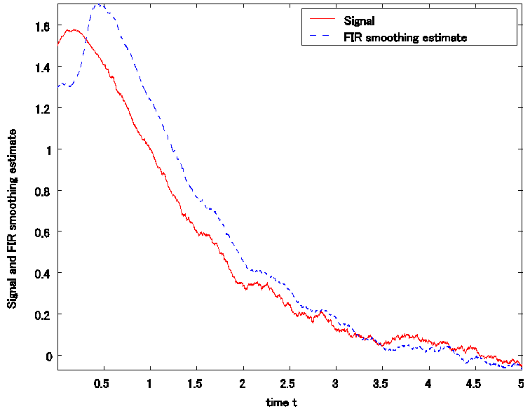
Figure 1. Signal and RLS-FIR smoothing estimate for white observation noise .

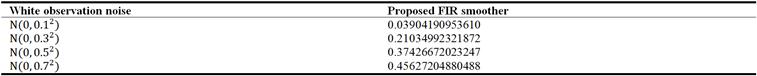
smoothing estimate  vs. , , for the white Gaussian observation noise . Here, the value of the finite-time interval  in the RLS-FIR smoother is  and the signal  at the start time , with the observed values between  and , is estimated. From Fig. 1, it is seen that the RLS-FIR smoothing estimate approaches gradually the signal as time  advances. Table 1 compares the mean-square values (MSVs) of the current FIR smoothing errors, , , with those by the RLS-FIR filtering errors [14], , for the observation noises , ,  and . Table 1 indicates, for both the FIR smoothing and filtering estimates, as the variance of the observation noise becomes small, the estimation accuracies are improved. Also, From Table 1, the estimation accuracy of the proposed RLS-FIR smoother is inferior to the RLS-FIR filter [14]. Table 2 shows the MSVs of the current FIR smoothing errors,, for the observation noises , ,  and . In Table 2, the MSVs are calculated based on 4500 number of FIR smoothing errors for the signal , , and . Whereas in Table 1, 2000 number of FIR smoothing errors are used for , . Table 3 shows the MSVs of the current FIR smoothing errors,, for the observation noises , ,  and . Here, . In comparison of Table 2 for the finite-time interval  with Table 3 for , the estimation accuracy of the proposed FIR smoother in Table 2 is preferable to that in Table 3. This might be based on the fact that, in the case of the finite- time interval the RLS-FIR smoother uses twice number of the observed values in calculating each FIR smoothing estimate recursively in contrast with . Table 4 shows the MSVs of the FIR

Table 1. Mean-square values of the current FIR smoothing errors and FIR filtering errors by [14] in terms of 2000 number of estimation errors for , .

Table 2. Mean-square values of 4500 number of FIR smoothing errors for , .

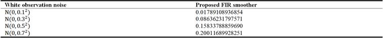
Table 3. Mean-square values of 4500 number of FIR smoothing errors for , .

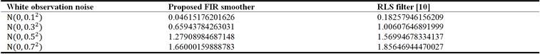
smoothing errors, by the current smoother, in terms of 4500 number of estimation errors during  for the observation noises, ,  and . Here, the finite-time interval is . In comparison of Table 4 with Table 2, the estimation accuracy for the finite-time interval  in Table 4 is almost same as the case of  in Table 2. In Table 4, the MSVs of the filtering errors by the RLS-FIR filter [14] are also shown. The MSVs indicate that the estimation accuracy of the current RLS-FIR smoother is almost same as the RLS-FIR filter [14] for the finite-time interval . Table 5 compares the estimation accuracy of the proposed RLS-FIR smoother with the RLS filter [10] in terms of the MSVs. The MSVs are calculated by , , in the current FIR smoother, and  in the RLS filter [10] for the observation noises, ,  and . Table 5 indicates that the estimation accuracy of the proposed RLS-FIR smoother is superior to the RLS filter [10]. Since the FIR filter does not calculate the estimate for , compared with the RLS filter, the proposed RLS-FIR smoother is feasible in estimating the signal for the time interval.

Table 4. Mean-square values of the current FIR smoothing errors and FIR filtering errors by [14] in terms of 4500 number of estimation errors for , .

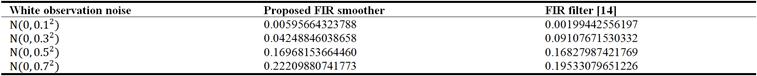
Table 5. Mean-square values of the current FIR smoothing errors and filtering errors by [10] in terms of 500 number of estimation errors for , .

For references, the state-space model, which generates the signal process, is specified by

6. Conclusions

In the RLS-FIR filter [14], the estimation of the signal process starts from the finite-time interval , hence the signal for the time interval, , is not estimated. From the reason to be able to estimate the signal for the time interval, , this paper, as a first attempt, proposes the RLS-FIR smoother, which estimates the signal at the start time of the finite-time interval  in linear continuous-time stochastic systems. The numerical simulation example has shown that the current RLS-FIR smoother is feasible. Also, the algorithm for the RLS-FIR smoothing error variance function and the condition for the stability of the RLS-FIR smoother are shown.

The proposed RLS-FIR smoother has the following properties.

(1)    As the variance of the white observation noise becomes small, the estimation accuracy of the RLS-FIR smoother is improved.

(2)    In the simulation, the estimation accuracies of the proposed RLS-FIR smoother for the finite-time intervals  and  are almost same. Also, for  and , the estimation accuracy of the proposed RLS-FIR smoother is almost same as the RLS-FIR filter [14]. In addition, in the proposed RLS-FIR smoother, the estimation accuracies for  and  are superior to the case of .

(3)    Since the RLS-FIR filter [14] does not calculate the estimate for , compared with the RLS filter [10], from the point of the estimation accuracy, the proposed RLS-FIR smoother is feasible in estimating the signal for the time interval.

Appendix Proof of Theorem 1

From the auto-covariance function (3) of the signal in the semi-degenerate kernel, (8) is rewritten as

(A-1)

Let us introduce an auxiliary function , which satisfies

         (A-2)

From (A-1) and (A-2), we obtain an expression for the optimal impulse response function

                      (A-3)

Differentiating (A-2) with respect to , we have

                           (A-4)

From (3), for ,  is valid. Hence, (A-4) is rewritten as

                      (A-5)

Let us introduce an auxiliary function , which satisfies

                                                   (A-6)

From (A-2) and (A-6), we obtain

                                          (A-7)

In a similar manner, differentiating (A-6) with respect to  and using (A-2) and (A-6), we obtain

                                          (A-8)

Putting  in (A-2), we have

                                                           (A-9)

From (3), in (A-9),  is valid for . Introducing a function

                                                                     (A-10)

we obtain (10). Similarly, putting  in (A-2), and introducing a function

                                                                     (A-11)

we obtain (12).

Putting  in (A-6), we have

(A-12)

From (3), in (A-12),  is valid for . Introducing a function

                                                          (A-13)

we obtain (11). Similarly, putting  in (A-6), and introducing a function

                                                          (A-14)

we obtain (13).

Differentiating (A-10) with respect to , we have

                            (A-15)

Substituting (A-7) into (A-15) and using (A-10) and (A-13), we obtain (16).

Differentiating (A-13) with respect to , we have

                            (A-16)

Substituting (A-8) into (A-16) and using (A-10) and (A-13), we obtain (17).

Differentiating (A-11) with respect to , we have

                            (A-17)

Substituting (A-7) into (A-17) and using (A-11) and (A-14), we obtain (18).

Differentiating (A-14) with respect to , we have

                            (A-18)

Substituting (A-8) into (A-18) and using (A-11) and (A-14), we obtain (19).

Substituting (A-3) into (4), we have

                                          (A-19)

Introducing a function

                                                        (A-20)

we obtain (9) for the FIR smoothing estimate .

Differentiating (A-20) with respect to , we have

                                 (A-21)

Substituting (A-7) into (A-21) and introducing

                                                       (A-22)

we obtain (14). Similarly, differentiating (A-22) with respect to , we have

                                (A-23)

Substituting (A-8) into (A-23), and using (A-20) and (A-22), we obtain (15).

From (A-10), the initial condition on the differential equation for  at  is given by

                   (A-24)

Corresponding to , we introduce, from (A-2), a function , which satisfies

      (A-25)

Here, we note that . Hence, we introduce

(A-26)

In (16), the initial condition  is given as the value of  at . Let us differentiate (A-25) with respect to .

   (A-27)

Let us introduce an equation, which  satisfies

  (A-28)

Taking into account of the auto-covariance function  in (3) for  and using (A-28), we obtain

(A-29)

Differentiating (A-26) with respect to , we have

   (A-30)

Substituting (A-29) into (A-30) and introducing

  (A-31)

we obtain (24) for  with the initial condition .

Differentiating (A-31) with respect to , we have

  (A-32)

Differentiating (A-28) with respect to , we have

  (A-33)

Taking into account of the auto-covariance function  in (3) for  and using (A-28), we obtain

(A-34)

Substituting (A-34) into (A-32) and using (A-31), we obtain (25) for  with the initial condition .

From (A-11), the initial condition on the differential equation for  at  is given by

(A-35)

Corresponding to , we introduced, from (A-2), a function , which satisfies (A-25). Here,  is valid. Hence, we introduced

(A-36)

In (18), the initial condition  is given as the value of  at .

Differentiating (A-36) with respect to , we have

  (A-37)

Substituting (A-29) into (A-37) and introducing

(A-38)

we obtain (26) for  with the initial condition .

Differentiating (A-38) with respect to , we have

(A-39)

Substituting (A-34) into (A-39), we obtain (27) for  with the initial condition .

Putting  in (A-25), we have

  (A-40)

From (3), , , is valid. From (A-26), we obtain (20).

Putting  in (A-28), we have

   (A-41)

From (3), , , is valid. From (A-31), we obtain (21).

Let us introduce a function

(A-42)

Differentiating (A-42) with respect to , we have

  (A-43)

Substituting (A-29) into (A-43), we obtain (22).  is given as the initial condition of (14) for  at . Here,  is given by

(A-44)

Differentiating (A-44) with respect to , we have

(A-45)

Substituting (A-34) into (A-45), we obtain (23).  is given as the initial condition of (15) for  at .

(Q.E.D.)

References

1. Kwon, W. H. and Kwon, O. K. (1987). FIR filters and recursive forms for continuous time-invariant state-space models, IEEE Trans. Automatic Control, 32 (4): 352–356.
2. Jazwinski, A. H. (1968). Limited memory optimal filtering, IEEE Trans. Automatic Control, 13 (5): 558–563.
3. Schweppe, F. C. (1973). Uncertain Dynamic Systems, Prentice-Hall, Englewood Cliffs,
4. N. J. Bruckstein, A. M. and Kailath, T. (1985). Recursive limited memory filtering and scattering theory, IEEE Trans. Information Theory, 31 (3): 440–443.
5. Kwon, W. H., Kim, P. S. and Park, P. G. (1999). A receding horizon Kalman FIR filter for linear continuous-time systems, IEEE Trans. Automatic Control, 44 (11): 2115–2120.
6. Han, S. H. Kwon, W. H and Kim, P. S. (2001). Receding-horizon unbiased FIR filter for continuous-time state-space models without a priori initial state information, IEEE Trans. Automatic Control, 46 (5): 766–770.
7. Kwon, W. H., Kim, P. S. and Park, P. G. (1999). A receding horizon Kalman FIR filter for discrete time-invariant systems, IEEE Trans. Automatic Control, 44 (9): 1787–1791.
8. Ahn, C. (2008). New quasi-deadbeat FIR smoother for discrete-time state-space signal models: an LMI approach, IEICE Trans. Fundam. Electron. Commun. Comput. Sci., vol. E91-A (9): 2671–2674.
9. Ahn, C. K. and Han, S. H. (2008). New  FIR smoother for linear discrete-time state-space models, IEICE Trans. Commun., E91-B (3): 896–899.
10. Nakamori, S. and Sugisaka, M. (1977). Initial-value system for linear smoothing problems by covariance information, Automatica, 13 (6): 623–627.
11. Nakamori, S. (2009). RLS fixed-lag smoother using covariance information in linear continuous stochastic systems, Appl. Math. Model., 33 (1): 242–255.
12. Nakamori, S. (2007). Design of extended recursive Wiener fixed-point smoother and filter in discrete-time stochastic systems, Digital Signal Processing, 17 (1): 360–370.
13. Nakamori, S. (2010). Design of RLS Wiener FIR filter using covariance information in linear discrete-time stochastic systems, Digital Signal Processing, 20 (5): 1310-1329.
14. Nakamori, S. (2013). Design of RLS-FIR filter using covariance information in linear continuous-time stochastic systems,Applied Mathematics and Computation, 219: 9598-9608.
15. Nakamori, S. (2014) Design of RLS Wiener FIR fixed-Lag smoother in linear discrete-time stochastic systems,CiiT International Journal of Programmable Device Circuits and Systems, 6 (8): 233-243.
16. Sage, A. P., Melsa, J. L. (1971). Estimation Theory with Applications to Communications and Control, McGraw-Hill, New York.
17. Kagiwada H. H. and Kalaba, R. E. (1968). Verification of the invariant imbedding method for certain Fredholm integral equations, Journal of Mathematical Analysis and Applications,. 23 (3): 540-550.
18. Kagiwada, H. H., Kalaba, R. E. and Vereeke, B. J. (1968). The invariant imbedding numerical method for Fredholm integral equations with degenerate kernels, Journal of Approximation Theory, 1 (3): 355-364.
19. Casti, J. L. and Kalaba, R. E. (1970). Proof of the basic invariant imbedding method for Fredholm integral equations with displacement kernels. Part II, Information Sciences, 2 (1): 69-76.
20. Bellman, R. and Ueno, S. (1973). Invariant imbedding and the resolvent of Fredholm integral equation with composite symmetric kernel, Jounal of Mathematical Physics, 14: 1489-1490.
21. Kagiwada, H. H., Kalaba, R. E. and Schumitzky, A. (1969). A representation for the solution of Fredholm integral equations, Proc. Amer. Math. Soc., 23: 37-40.
22. Kagiwada, H. H. and Kalaba, R. E. (1975). Integral Equation via Imbedding Methods, Addison-Wesley.
23. Koshel, K. V., Ryzhov, E. A. and Zyryanov (2014). V. N., A modification of the invariant imbedding method for a singular boundary value problem, Communications in Nonlinear Science and Numerical Simulation, 19 (3): 459-470.