Features of Active Particle Brownian Walk Dynamics Excited by White Noise in Media with Non-Linear Friction Which Value Depends Partially on Particle Vivacity Level

Vladimir A. Dobrynskii^*

Institute for Metal Physics of N.A.S.U., Kiev, Ukraine

Abstract

It is known a long time (about one century ago) that there is a phenomenon of "tunnelling", i.e. passage of low-energy elementary particles through an energetic barrier that ones could not surmount classically. Explanation of the phenomenon is made in the quantum mechanic framework using the Heisenberg uncertainty principle. The phenomenological model presented here permits to explain the given phenomenon in the classic physics framework provided that the particles interact with a space-time continuum. In other words, in the model, it is assumed that both the particles and 1-dimensional medium where they make their Brownian walks under action of "white" noise are active and do interact each other. We assume additionally that the noise influence on the particles dynamics is much deeper than simple stimulating of the Brownian walks and consists in changing of the internal particle status (property) calling by vivacity. Under such the assumptions a few active particles increase the vivacity so much to penetrate over the impermeable friction barrier and to run in the positive half-axis depth, i.e. to "tunnel" in domains which are situated behind the aforesaid barrier. Making a series of snapshots of 1-dimensional frequency distribution function of an ensemble of particles we are convinced in the aforesaid.

Keywords

Active Particle, Vivacity, Natural Internal Frequency, Frequency Distribution Function

Received: June 15, 2016
Accepted: July 29, 2016
Published online: September 23, 2016

@ 2016 The Authors. Published by American Institute of Science. This Open Access article is under the CC BY license. http://creativecommons.org/licenses/by/4.0/

1. Introduction

It is known a long time (about one century ago) that there is a phenomenon of "tunnelling", i.e. passage of low-energy elementary particles through an energetic barrier that ones could not surmount classically. Explanation of the phenomenon is made in the quantum mechanic framework with aid of the quantum particle tunnelling using the Heisenberg uncertainty principle. The 1-dimensional Schrödinger equation is used as a mathematical foundation for the quantum tunnelling explanation (see, e.g., [11, 12]).

The phenomenological toy model presented here permits to explain the given phenomenon in the classic physics framework only but provided that the particles do interact with a space-time continuum. In other words, in the model under consideration, it is assumed that both the particles and 1-dimensional medium where they make their Brownian walks under action of "white" noise are active and do interact each other. We assume additionally that the noise influence on the particles dynamics is much deeper than simple stimulating of the Brownian walks and consists in changing of the internal particle status (property) calling by vivacity. Under such the assumptions a few active particles increase the vivacity so much to penetrate over the impermeable friction barrier and to run in the positive half-axis depth, i.e. to "tunnel" in domains which are situated behind the aforesaid barrier.

To be precise, to give one of possible explanations for the so-called "tunnel penetration" of low energy particle through the energetic barrier in the classic physics framework and to clear up a mechanics which may stay behind for surmounting of the aforesaid barrier by separate particles we propose a conception of "active" particles and create a stochastic phenomenological mathematical model of their behaviour which appears and develops as a result of the environment white noise action on them. As against usual (passive) particles the active ones possess the more numerous characteristic set than that of the usual ones and includes additionally two unobservable characteristics which we propose to call "vivacity" and "natural internal frequency". On existence of such kind characteristics of the particle one should guess observing results of simulation of the Brownian particle walk dynamics. As we are convinced later a presence of these characteristics allows single selected active particles to visit such space domains which are always closed for visiting by the usual "passive" ones. The latter ones can visit the aforesaid domains never.

As a whole a problem of how determinism and chance interplay each other in nature phenomena stays one of the most important fundamental questions standing in front of science up till now. Widespread systematic investigations directed to research the given problem are started recently relatively. In doing so random walk researching is making both in random and non-random environments [1]. Investigations showed to researchers’ surprise that a stochastic action of random noise stabilizes behaviour of system dynamics rather than insets chaos inside it very often [2-4]. There are a lot of references (see, e.g., [5-7]), where influence of noise on the periodically forced particles dynamics and their Brownian random walk are studied separately. A usual approach to examine an impact of fluctuations on the particles dynamics consists in that to include in an ordinary differential equation systems that describe it terms which generate or multiplicative or additive noise rather than both ones. However one aspect of the problem ― what is a sort of particles which the noise acts on,― as far as we know, was never considered early. As for us, we think the every particle possesses a certain feature peculiar to this particle, something like its natural internal frequency. If the given frequency is equal to zero, then the particle under consideration is usual (or passive) otherwise the one is active. As will be seen further, the active and passive particles give a very distinct different response on the white noise action. Our approach for to study of the Brownian walk dynamics of the active particles that undergo a persistent action of the standard white noise consists in simulation of this dynamics with aid of two ordinary stochastic differential equation system. The first system equation describes the active particle Brownian walk dynamics along the space axis and the second one allows us to describe how the active particle vivacity changes under influence of the white noise impulses. We assume in doing so that space resistance to a particle movement depends on not only of the space point but the particle internal status too. This assumption does not contradict the modern physical ideas. Studies of the present article continue (or, to be more precise, lie in a bed of) those in [8-10].

2. Mathematical Model

Creating the mathematical model of the particles dynamics we assume that i) they do not interact one another; ii) dynamics of any particle controls by the same system of stochastic ordinary differential equations. Anyway we research numerically solutions of the following system of stochastic ordinary differential equations:

,     (1)

.

Here  be the space particle co-ordinate, be its vivacity, , and  be its natural internal frequency. By  is denoted the standard Wiener’s process yielding the standard white noise. The particle is called active when and passive otherwise, i.e. when . Other parameters all are constants. In doing so , , . As for values of , we consider, as a rule, . One more, analysing the term characterizing a medium resistance to the Brownian particle walk we want to notice that its main feature is dynamical dependence on . This yields a phenomenon of very different medium resistance at the same medium point to moving of particles having different vivacity. In doing so if , then the more the particle vivacity the more the medium resistance to its moving at the given space point and vice versa: if , then the more the particle vivacity the less the medium resistance to its Brownian walk at the same point. The latter can lead to appearance of single active particles that can penetrate much deeper inside positive semi-axis of  than the other ones. As we shall see further such kind events occur in fact. Let us pay attention also to that although the vivacity we take for characterizing of the active particle properties is a parameter artificial enough and, say, its energy (which is equal to  for the particle with mass of 1) is much more natural one nevertheless we use the former rather than latter because the vivacity allows us to illustrate better how the particles and media interact each other and change their properties in doing so.

In order to find the experimental frequency distribution function we solved Eq. (1) as Ito’s process associated with the given equation system. As initial conditions we take, usually, , where , ,, and  always. We consider a set consisting of 3072 particles and find its Brownian walk way for times from  until to . After completion of every Ito’s process, in order to watch for changing of the experimental frequency distribution function shape we form a number of snapshots which pick up an instant view of the aforesaid function at certain times. Usually they are . But sometimes, in order to monitor changing of the distribution function shape in more details, we took the snapshots in various different .

First to start a discussion of the simulation results we should attract reader’s attention to that the results under review below are a little fraction of all those we have and are picked out for presentation here as the most informative ones. For example, the first two series of histograms that are analysed in section 3 are computed for the initial . However numerical experiments were done with the very same parameter set values for  and  also. In doing so the results obtained in the former case turn out to be more trivial than those for . As for the latter case, we do entirely not obtain graphical figures because numerical computations were cancelled at  due to underflow or overflow. Analysis of data that accompany a cancellation of the computations show that, in the case with in doing so, the Brownian walk of the particle set are much more intensive than that started from the point  and hence its development data achieve those of the latter for times much less than  rather than only . Beyond  the Brownian particle set walk intensiveness becomes so huge that exceeds our possibility to its computation. The latter yields in turn either both the numerical computation underflow and overflow or someone of them. Concluding what is the aforesaid we would like to call reader’s attention to that conclusions we make lean always on all totality of our knowledge (including the knowledge obtained in the numerical experiments whose results do explicitly not shown in the article) rather than only analysis of the histogram series that are presented in section 3 below. We want to notice reader’s attention to this matter one more.

3. Simulation Result Analysis

In order to improve and simultaneously to simplify the presentation we will use two the histogram kinds which one permits us to look at for the Brownian walk of small enough fraction of the particles (it can consist of alone particle even) and the other permits us to watch for the Brownian walk of the most particles of. Analysing graphics (which are not included in the text) of the experimental distribution function, otherwise, probability of presence of the particle set to the left of some point of the axis in order to confirm time and again the following important observation: the probability of presence of the particle set to the left of the starting (initial) point  is equal to  always.

At first to start analysing of the first two series of histograms presented below we should explain that a choice of  is not accidental there. Because before to make computations with this initial value we made already numerical experiments for the same parameter values and initial data equal to  and . The results are different. Namely: the computations with  were successfully fulfilled for all times from  till . However their results are trivial in a sense because yield the functions under study of expected look. As for the experiments with , they were not finished because the computations were cancelled due to both underflow and overflow. In light of the said above the choice  seems to be natural. We consider the two series of histograms that are computed with the same but one parameter values. Both Ser. 1 and Ser. 2 figures are found with the same but one parameter values and initial data. The ones are the following: , . However the values of  are different there. Namely:  in Ser. 1 and  in Ser. 2. Let us analyse graphs presented in Ser. 1 and Ser. 2 in detail. Before to start analysis of graphs presented below let us notice that, due to restriction on the article size, we are forced to exclude a number of low-informative ones, and to restrict ourselves by considering of the graphs that confirm our conclusions. As for the graphs excluded from the text, they presented beginning stages of developing of 1-dimensional frequency distribution function for the active particles. These are either the bell-like functions or the ones presented below but their right side, where we watch appearance of the separate active particles that "tunnel" in deepness of the positive axis half, i.e. similar to those are shown in Fig. 1 of Ser. 1, Fig. 11 of Ser. 3, etc.

Considering the histograms shown in Figs. 1-4 of Ser. 1 we can easily watch how the tunnelling active particles appear and move in deepness of the positive axis half in the course of the while [186, 248]. In the latest times, as it is well-seen from Fig. 4 (of Ser. 1) histogram, the particle walk distance scale in the positive axis half is much more expansive than that in the negative axis half although, the biggest fraction of the particle set concentrates near the particle its point. In doing so, the latter said (particle set concentration near the start point) is true for all times. Comparing the aforesaid frequency distribution functions with those presented in Figs. 6-9 of Ser. 2 one can find that they look on the whole similar. Although there are visible distinguishes between them, of course. First, at  in Ser. 2, there already exists the active particle tunnelling into the positive axis half. At , we observe two such the kind particles already while, in Ser. 1, we can watch two distinctly observable such the kind particles at time  only. In doing so, in the latest observable times, on the contrary, the particle walk distance scale in the negative axis half is much more expansive than that in the positive axis half. Considering the histograms shown in Figs. 1-4 of Ser. 1 and Figs. 6-8 of Ser. 2 one can easily see also that a number of the particles that own such kind of the Brownian walk and penetrate very far away to the right from their initial position is essentially less than that of particles that go far away to the left from their initial position. However in Ser. 2 as in Ser. 1, the most fraction of the particles makes its Brownian walk in relatively small vicinity of the start point always. This is well-seen from Fig. 9 of Ser. 2. One more remark is. Besides a presentation of final distribution of the particles in the axis, the histogram in Fig. 10 of Ser. 2 bears one more very important information which we should tell a reader. Namely: the observant reader noticed of course that although we declare making computations for times  (and that we really make always) however usually we show numerical experiment results for times that is less (sometimes considerably) than . This is connected not with the results themselves but with their numerical values that exceed possibilities of data presentation system we have to show the ones in a suitable form. Data obtained in the second series at  and presented in view of the histogram on Fig. 10 of Ser. 2 are critical in the sense that this kind histogram gives some information respecting of the Brownian walk limits still while another its kind in the case under scrutiny (so-called the s-histogram) is practically non-informative and therefore is not presented here.

Summing up of consideration of the histograms presented in Series 1-2 we can formulate the following infers:

I)       up to the certain time, the Brownian walk dynamics of the active particle set does not differ from that of the passive one set;

II)    starting of the time mentioned above, one can observe visible differences in the aforesaid dynamics, namely: in the former one, there particles appear that begin to move in deepness of positive half of the axis;

III)  the active particles penetrating over the highest friction barrier are a very few always (in the numerical experiments, we watched one-two-three but never more of such the kind ones), i.e. a probability of appearance of the phenomenon under examination is close enough to zero (although the phenomenon itself is observable!);

IV)  a number of the active particles penetrating in deepness of the negative half of the axis is considerable, in particular, it is well-seen from the histograms under examination that a probability of existence of such the kind ones is strong more than zero;

V)     the most fraction of the particles make their Brownian walk in vicinity of their start point, i.e. with probability close to 1, in all times, one can find almost any active particle in vicinity of its start point.

The next three series of the numerical experiments are devoted to specify how the results pointed out above depend on varying of the model parameters. Before to begin analysing these series of graphs in detail, let us make infers which are evident from the first glance. First, the appearance of the penetrating active particles takes place near by , i.e. at sufficiently far away times. Second, even though the model parameters are close enough, dynamics of displacement of the penetrating active particles in deepness of the positive half-axis can differ very much.

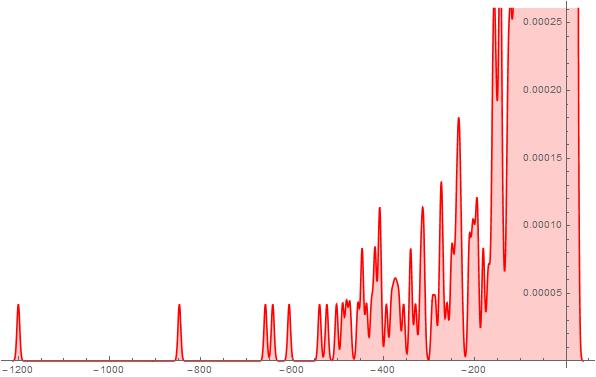
Figure 1. S-Histogram of the 1-dimensional frequency distribution function at t=186. (Ser. 1).

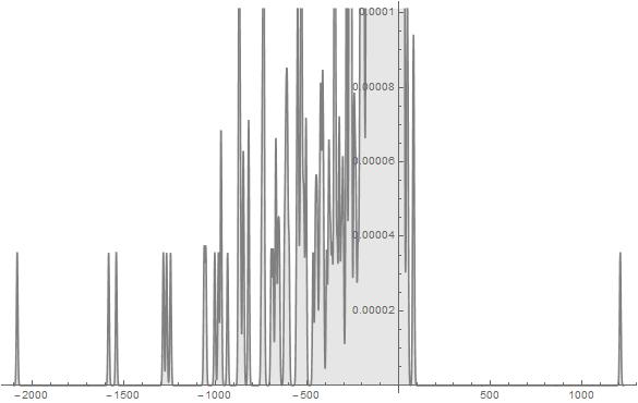
Figure 2. S-Histogram of the 1-dimensional frequency distribution function at t=236. (Ser. 1).

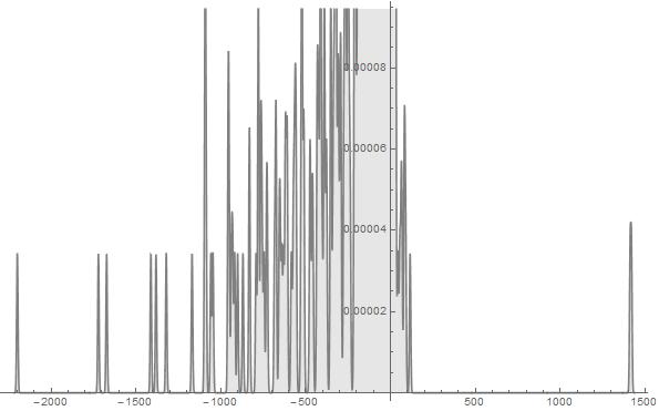
Figure 3. S-Histogram of the 1-dimensional frequency distribution function at t=242. (Ser. 1).

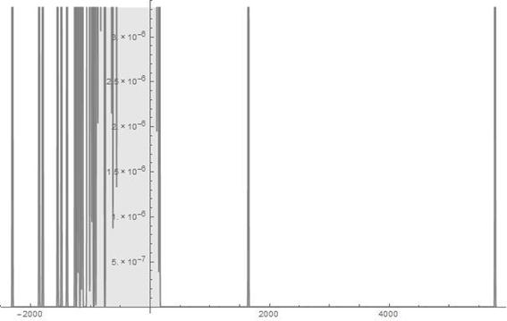
Figure 4. S-Histogram of the 1-dimensional frequency distribution function at t=248. (Ser. 1).

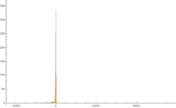
Figure 5. Histogram of the 1-dimensional frequency distribution function at t=248. (Ser. 1).

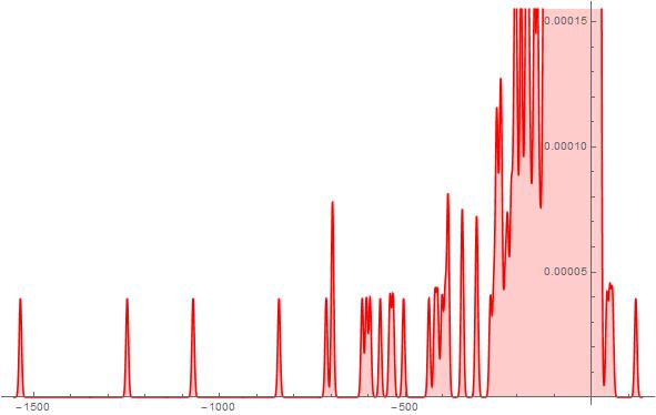
Figure 6. S-Histogram of the 1-dimensional frequency distribution function at t=186. (Ser. 2).

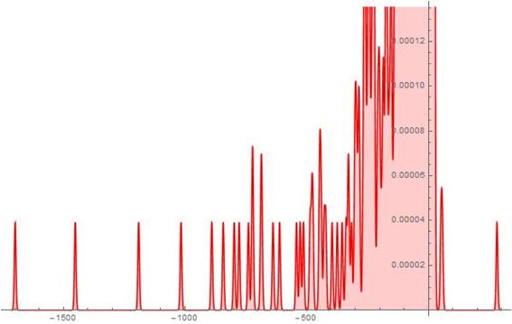
Figure 7. S-Histogram of the 1-dimensional frequency distribution function at t=200. (Ser. 2).

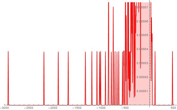
Figure 8. S-Histogram of the 1-dimensional frequency distribution function at t=215. (Ser. 2).

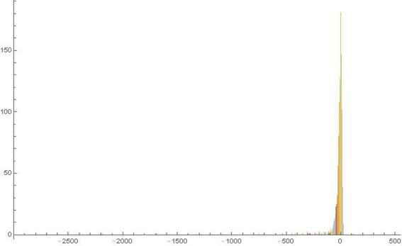
Figure 9. Histogram of the 1-dimensional frequency distribution function at t=215. (Ser. 2).

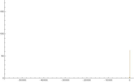
Figure 10. Histogram of the 1-dimensional frequency distribution function at t=220. (Ser. 2).

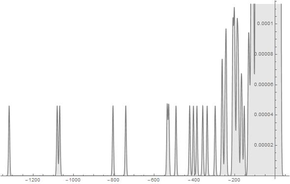
Figure 11. S-Histogram of the 1-dimensional frequency distribution function at t=194. (Ser. 3).

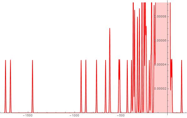
Figure 12. S-Histogram of the 1-dimensional frequency distribution function at t=216. (Ser. 3).

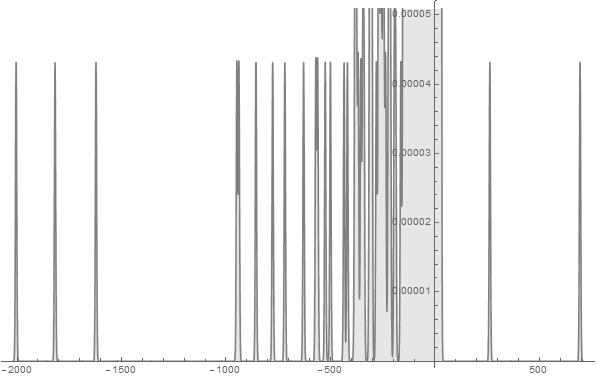
Figure 13. S-Histogram of the 1-dimensional frequency distribution function at t=224. (Ser. 3).

Figure 14. S-Histogram of the 1-dimensional frequency distribution function at t=236. (Ser. 3).

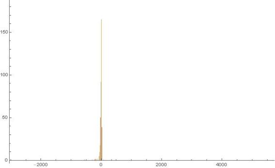
Figure 15. Histogram of the 1-dimensional frequency distribution function at t=248. (Ser. 3).

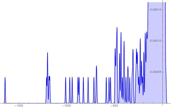
Figure 16. S-Histogram of the 1-dimensional frequency distribution function at t=202. (Ser. 4).

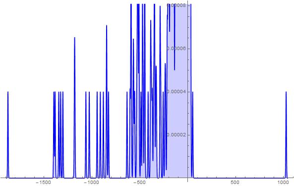
Figure 17. S-Histogram of the 1-dimensional frequency distribution function at t=212. (Ser. 4).

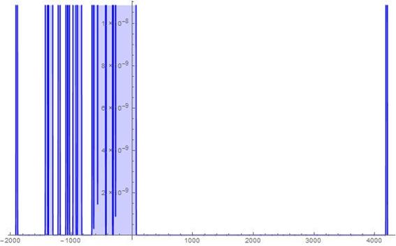
Figure 18. S-Histogram of the 1-dimensional frequency distribution function at t=213. (Ser. 4).

Figure 19. Histogram of the 1-dimensional frequency distribution function at t=213. (Ser. 4).

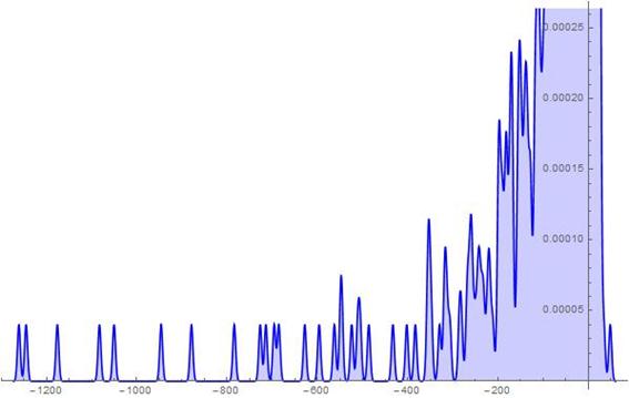
Figure 20. S-Histogram of the 1-dimensional frequency distribution function at t=194. (Ser. 5).

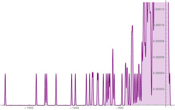
Figure 21. S-Histogram of the 1-dimensional frequency distribution function at t=202. (Ser. 5).

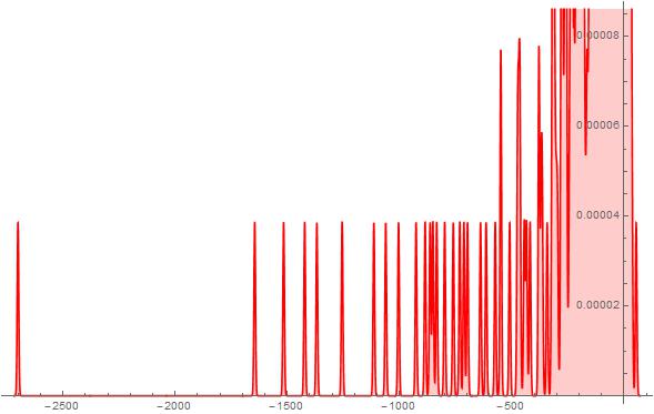
Figure 22. S-Histogram of the 1-dimensional frequency distribution function at t=212. (Ser. 5).

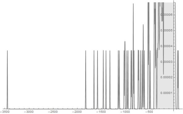
Figure 23. S-Histogram of the 1-dimensional frequency distribution function at t=220. (Ser. 5).

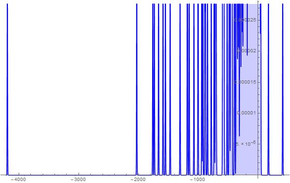
Figure 24. S-Histogram of the 1-dimensional frequency distribution function at t=228. (Ser. 5).

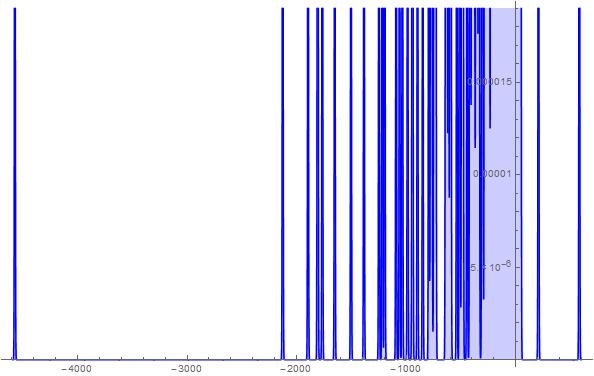
Figure 25. S-Histogram of the 1-dimensional frequency distribution function at t=232. (Ser. 5).

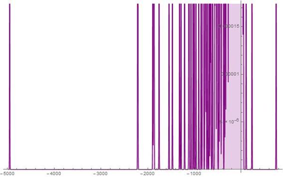
Figure 26. S-Histogram of the 1-dimensional frequency distribution function at t=236. (Ser. 5).

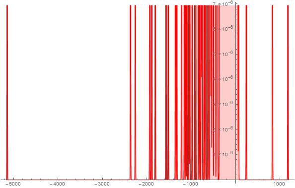
Figure 27. S-Histogram of the 1-dimensional frequency distribution function at t=238. (Ser. 5).

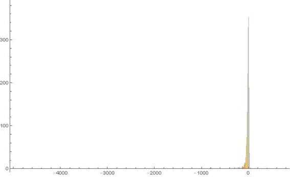
Figure 28. Histogram of the 1-dimensional frequency distribution function at t=238. (Ser. 5).

Let us consider the aforementioned series in detail now. Our first step is to study a dependence of the Brownian particles set walk dynamics behaviour on . Situation we have here is not simple. First of all we should tell that considerable increasing of its value, say, up to  leads to a practically instant cancellation of numerical experiment due to overflow/underflow. Moreover, even respecting modest increasing of , say, to  can yield (and yields really but in later times) the aforesaid cancellation. As for values of  that vary nearby 900, we tried to find the upper limit initial data  which provide penetration of a few particles far away to the right for the time under examination. In order to do this, we made some of the numerical experiments with the same parameter values as those in Ser. 1-2 and found that the limit under seeking is  approximately. Ser. 3 graphs confirm the just said indirectly. They show the numerical experiment results computed with ,  and .

Comparing Ser. 3 histograms with those of Ser. 1 one can see at once that after the appearance of active particles which begin to penetrate to the right axis half (that happens in Ser. 3 at time some less than ) the Brownian walk dynamics of the aforementioned particles are distinctly different than that in Ser. 1-2 because these particles penetrate in depth of the right half of the axis considerably quicker than those in Ser. 1-2. In doing so, in the end of observable times, we find that their penetration in the right axis half is considerably deeper than that of the rest of particles set in the left axis half. In order that to be convinced in validity of the aforesaid, one should compare scales presented in Figs. 12-14 or, better, in Fig. 15 of Ser. 3. A propos, the histogram in the last figure of the just enumerated shows that nevertheless the wide walk interval (the one extends from  to more than ) the most fraction of the particles set concentrates near byall the same.

The last histogram series are devoted to study of how much dynamics of the Brownian particle walk depends on the model parameters, or to be more precise, on  which is principal among the parameters and its value defines influence bulk that the vivacity exerts on ability of the particles to penetrate through the highest friction barrier. In Ser. 4 and Ser. 5, the value of  will be stated equal to  and  respectively. These values are more than that fixed in Ser. 3 in two and four times respectively. A main result of numerical experiments fulfilled with these values of  consists in continuation of presence of scenario of the Brownian particles set walk that is described above. However a realization of the given scenario takes place for the different initial (start) points, namely: ,  for Ser. 4, Ser. 5 respectively while, in Ser. 3,  only. Summarizing up all what is just said above we can make a conclusion that increasing of values of  towards 0 does not cancelled the existence of the Brownian particles set walk scenario that provides appearance of the active particles penetrating in domains situated behind the highest friction barrier as well as further development of the given tunnelling. However this scenario realizes with the different initial data for  which must decrease (and do really) with increasing of . After this principal sentence we infer, examining results shown in Ser. 4-5 figures let us tell that the parameter values used here for making computations are the following:,  are the same for Ser. 4-5 but is different. Namely:  for Ser. 4 and  for Ser. 5. Comparing these parameter values with analogous ones in Ser. 3 one can see that the values of  are more than that in Ser. 3 in two and four times respectively and the value of  is more slightly than that in Ser. 3. As for , its values are pointed out above. As we mentioned already increasing of  under keeping of the rest parameter values results, as a rule, in increasing of . However, results of the numerical experiments under review show that if simultaneously with increasing of  to increase  to the numbers pointed out above, one can easily observe then that the aforesaid phenomenon does not take place at all and, on the contrary, the values of  have to be decreased.

Let us now analyse the graphs presented in Ser. 4-5 in detail. In Fig. 16 of Ser. 4, there is presented the 1-dimensional frequency distribution function at  showing that the Brownian particles set walk dynamics develops in the depth of the negative axis half and there are not the active particles penetrating into the positive half-axis. After that time we pick up the appearance of a very few particles that walk far off inside the positive axis half. We want to notice attention on an extreme fewness of the aforesaid particles once more and to stress that their number may be, as is well-seen from the histogram in Figs. 17-18 of Ser. 4, even 1 or 2. However these few particles penetrate in the depth of the positive axis half considerably far off then the ones that walk in the depth of the negative axis half. A propos, as is well-seen from the histogram in Fig. 18 of Ser. 4, a number of the latter particles is much more than that of the former ones. Simultaneously the histogram in Fig. 19 of Ser. 4 shows nevertheless that the most particles make their Brownian walk near by their initial position. Considering the histograms shown in Figs. 20-27 of Ser. 5 which are similar in general the ones in Figs. 16-18 of Ser. 4 one can easily see that, up to , the Brownian particles set walk dynamics is trivial in a sense that it develops in the depth of the negative axis half and there are not the active particles tunnelling into depth of the positive half-axis. After that time we pick up the appearance of a very few particles that walk far off inside the positive axis half. We can see again an extremely fewness of such the kind particles here. However their penetration in the depth of the positive axis half is considerably less then that of the particles that walk in the depth of the negative axis half. Furthermore the histogram in Fig. 28 of Ser. 5 confirms once more the fact stated already that the Brownian walk of the most particles concentrates near by their initial position under any circumstances.

4. Conclusions and Speculations

Before to make final conclusions from all what is the aforesaid we should attract the reader attention to that all the simulations are fulfilled with aid of a notebook and thus its computational possibilities confined us in making numerical experiments. In particular, 3072 being a number of particles under study and 248 being a time of observation are quantities extremely close to limit for this notebook to make computations described above. Nevertheless it is not able to prevent us to make entirely substantiated conclusions for dynamics of the Brownian walk for sets having more than 3072 particles for times more than 248. After this preface we are ready to formulate principal sentences.

First of all we won’t repeat the conclusions I)-V) as well as ones we make respecting influence of values of the parameters  and  on the active particle Brownian walk dynamics as well as the conditions of appearance of the active particles overcoming the highest friction barriers and tunnelling into the domains lying behind the barriers. Instead this we would analyse how much for the assumptions we made in process of creating the model under scrutiny are agreed with properties which might and do possess a real space-time as well as elementary particles. Our main assumptions (excluding standard ones respecting the "white" noise and the Brownian walk dynamics) are as follows.

I.     Dynamics of the Brownian active particle walk which appears and develops due to the white noise action differs distinctly of that for the passive one. A main feature distinguishing the former from the latter consists in appearance of a very few particles which can overcome the highest friction barriers and penetrate in domains lying beyond the barriers.

II.   Ability of the active particle to accumulate its vivacity (i.e. possibility to overcome the friction barrier) depends on the internal active particle status, in particular, on its characteristic which we call a natural internal frequency.

III.Principal condition providing of appearance of the active particles which can overcome the highest friction barriers and penetrate in domains lying beyond the aforesaid barriers is ability of medium where the particles make their Brownian walk to interact with those. In doing so one of its (medium) parameters must be analogous to the parameter , i.e. the one value must influence on the active particle ability to accumulate the vivacity immediately.

IV. Crucial condition for appearance of the active particles which tunnel though the highest friction barrier is a sign of  rather than its absolute value. In particular,  must be.

Obviously all the assumptions are, in general, in accordance with the modern physical ideas of properties which are inherent to the space-time continuum and elementary particles. A unique exclusion is a claim of sign-definiteness of . However, if to conjecture that, for instance, is a function  whose values fluctuate in time near by its mean value being equal to 0, the model under scrutiny can help then to realise, as a whole, for mechanics of how (cosmic) particles in process of only their mutual collisions can accumulate so much of energy that they penetrate through the highest energetic barriers.

References

1. Rěvěsz P. Random walk in random and non-random environments. World Scientific. Singapore, 1990.
2. Haken H. Synergetics. Springer. Berlin, 1983.
3. Haken H. Advanced synergetics. Springer. Berlin, 1985.
4. Zaslavsky G. M., Sagdeev R. Z., Usikov D. A. and Chernikov A. A. Weak chaos and quasi-regular patterns. Cambridge University Press, Cambridge, 1987.
5. Schuster H. G. Deterministic Chaos. Springer. 3^rd edition. Berlin, 1995.
6. Karatzas I. and Shreve S. E. Brownian motion and stochastic calculus, Springer. 2^nd edition. Berlin, 1996.
7. Vavrin D. M., Ryabov V. B., Sharapov S. A. and Ito H. M. Chaotic states of weakly and strongly nonlinear oscillators with quasiperiodic excitation. Phys. Rev E 53, 1996, pp. 103-114.
8. Ivanov M. A, Dobrynskiy V. A. Random walk of oscillator on the plane with non-homogeneous friction. Int. INFA-ANS J. Problems Nonlinear Analysis in Engineering Systems", vol. 12, no. 1 (15), 2006, pp. 101-116.
9. Ivanov M. A, Dobrynskiy V. A. Stochastic dynamics of oscillator drift in media with spatially non-homogeneous friction, J. Automation and Information Sci., vol. 40., no. 7, 2008, pp. 9-25.
10. Dobrynskii V. A. Unusual frequency distribution function shape generated by particles making Brownian walk along line with monotone increasing friction, Int. J. of Mathematics and Computation Sci., vol. 1., no. 3, 2015, pp. 91-97.
11. Walecka J. D. Topics in Modern Physic: Theoretical Foundations. World Scientific, 2013, 500 pp.
12. Razavy M. Quantum Theory of Tunneling. World Scientific. 2^nd edition, 2014, 792 pp.