A Step Towards Optimal Operation and Control of Batch Distillation Columns Using Reinforcement Learning

M. A. Mustafa^*

Department of Chemical Engineering, Faculty of Engineering, University of Khartoum, Khartoum, Sudan

Abstract

An important amount of work exists on the topic of optimal operation and control of batch distillation. Although previous efforts are still based on the assumption of an accurate process model being available, there will always remain the challenge of practical applications. Reinforcement Learning (RL) has been recognized already as a particularly suitable framework for optimizing batch process operation however no successful application to batch distillation has been reported. Thus, this paper presents RL as an automatic learning approach to batch distillation. Incremental batch to batch learning is demonstrated, for a range of case studies starting from a small initial training data set and with no assumption of prior knowledge of VLE. Furthermore the robustness of the RL algorithm, towards uncertainty in process variables, is demonstrated.

Keywords

Reinformcent Leanring, Batch Processes, Optimisation

Received: December 15, 2016
Accepted: January 17, 2017
Published online: February 28, 2017

@ 2016 The Authors. Published by American Institute of Science. This Open Access article is under the CC BY license. http://creativecommons.org/licenses/by/4.0/

1. Introduction

The rising importance of high-value-added, low-volume specialty chemicals has resulted in a renewed interest in batch processing technologies [1]. Batch distillation is an important and widely used separation process in batch process industry. Its main advantage, over continuous operation, is the ability to be used as a multi-purpose operation for separating mixtures into their pure components using a single column. Batch distillation can also handle a wide range of feed compositions with varying degrees of difficulty of separation (e.g. wide ranges of relative volatilities and product purities). Although the typical consumption of energy is more than in continuous distillation, more flexibility is provided with less capital investment [2]. Besides the flexibility in the operation of batch distillation columns, a range of challenging design and operational problems occur due to its inherent unsteady state nature.

2. Literature Survey

The main sequence of events in operating a batch distillation column starts with the feed charged into the reboiler. The column is then operated at total reflux until the column reaches steady state. This initial phase is known as the start-up phase. In the second phase, or production phase, light component product is collected into a product tank until its average composition drops below a certain specified value. This cut is referred to as the main cut (The 1^st main cut is sometimes preceded by taking off the low boiling impurities at a high reflux ratio). After that, the first intermediate distillate fraction (off-cut or slop cut) is produced and stored in a different tank. This procedure is repeated with a second main cut and second slop cut and so on until the concentration of the heaviest component, in the reboiler of the column, reaches a specified value. At the end of the batch, the operation of the distillation column goes through a shutdown phase. Slop cuts contain the material distilled, which does not meet specification. Considerable work in slop handling strategies has been reported in the literature [3, 4]. On the other hand, a totally different operating policy is the cyclic operation of a batch distillation column. In the case of a regular column, the cyclic operation could be characterised by repeating a three period operation [5]: Filling, Total Reflux, and Dumping.

The main manipulated variable, in the process of controlling a batch distillation column, is the reflux ratio. The frequently used and conventional approach towards controlling the operation of a batch distillation column, during the production of main cuts, is either to operate at constant reflux ratio or to operate at a varying reflux ratio (constant distillate composition). During operation at constant reflux ratio, the distillate composition is allowed to vary resulting in a simpler strategy and hence it is more commonly used in industry. The second approach is conducted by maintaining a fixed overhead composition while varying the reflux ratio. The two approaches used are simple but provide sub-optimal results. The second manipulated variable, in controlling a batch distillation column, is the boil-up rate: the quantity of liquid in the reboiler that is evaporated per unit time. In case of a batch distillation column, the boilup rate is often held at a maximum rate consistent with allowable vapour velocities and liquid capacities. In addition to the variables just mentioned, Farhat et al. [6] used the switching time for different cuts as an extra decision variable.

Throughout the literature, the formulation of the optimal control problem in batch distillation has been categorised as either a: Maximum Distillate Problem [7, 8]; Minimum Time Problem [9-13]; Maximum Profit Problem [14, 15]. Mujtaba and Macchietto [16] provided an efficient framework for on-line optimization of batch distillation with chemical reaction. The technique starts by finding optimization solutions to the batch distillation with chemical reaction problem, in order to solve the maximum conversion problem. The optimization was performed for a fixed batch time and given product purity. The maximum conversion, the corresponding amount of product, optimal constant reflux ratio, and heat load profiles were plotted for different batch times. Polynomial curve fittings were then applied to the results of the optimization and were used to formulate a non-linear algebraic maximum profit problem.

Mujtaba and Hussain [13] developed an optimization framework to tackle efficiently the optimal operation of dynamic process due to process/model mismatches. The method was applied to a batch distillation process where use is made of a neural network to predict the process/model mismatch profiles for the case study used. The Neural Network was then trained to predict the process/model mismatch, for each state variable, at the present discrete time. The mismatch then between the actual process/model (represented by error between rigorous model and simple model) and that predicted by the network was used as the error signal to train the Neural Network. The simple model was then used together with the Neural Network, to calculate the optimal reflux ratio to achieve the separation in minimum time. The results were then compared with the more rigorous model, which was used to represent the actual process in their case study. It was concluded that with the use of a simple model with mismatches, the optimal operation policy could be predicted quite accurately using the Neural Network. Although important work by Mujtaba et. al. [13, 16] reduces drastically the computational time used to solve differential equations, however exact knowledge of a mathematical process model is still assumed.

One of the first applications of Artificial Intelligence as the central part of batch distillation automation was by Cressy et al. [17]. They made use of Neural Networks in order to learn the control profiles of a batch distillation with a binary mixture: methanol and water. Two Neural Networks were used in the methodology: Neural Emulator (used to approximate the input/output function defined by the forward dynamics of the column) and a Neural Controller. The trained Neural Network achieved an error of less than 3% over a narrow range of conditions. Over a wider range, the results were not uniformly good. Furthermore, the amount of training data of 4080 training patterns would justify such a good fit to the observed data. The immediate concern is the issue of acquiring such an amount of data in practice.

Stenz and Kuhn [18] managed to integrate operator's knowledge, using fuzzy technology, into the automation of the batch distillation process. They concluded that fuzzy logic is not a superior method, but is rather an addition to the toolbox of the automation engineer, which is potentially useful. Although fuzzy logic presents the operator誷 know how as a sequence of acting steps, it still does not aim at giving the optimum solution. Wilson and Martinez [19] proposed a novel approach towards batch process automation involving simultaneous reaction and distillation. The methodology proposed combined fuzzy modelling and RL. The RL part of the methodology meant that the controller implemented is geared towards incrementally achieving goals, using rewards obtained as guideline. However, a large amount of data (1000 randomly chosen batches) is required for learning, which is well beyond the small number of initial batch runs that would be practically available in industry.

Further important work to determine efficient time profiles still depends upon having an accurate process model [20-23]. In practice such models are never available partly because conditions and parameters vary from one batch to another. Furthermore, the classical open loop time profile cannot react to measurements during the progress of a batch. The industry is faced with composition analyzers which are again often not available and seldom instantaneous [2]. Despite all those problems human operators have managed so far to incrementally drive those processes to near optimal operation.

The particular suitability of Reinforcement Learning (RL) as a framework for optimizing batch process operation has been recognized already [19, 24, 25]. The proposed hybrid predictive model (which form part of the RL algorithm) delivered adequate performance in previous applications to batch reactors, however difficulties were faced when applications to batch distillation where conducted by Mustafa and Wilson [26] who identified the predictive model to be crucial to the success of the RL algorithm. Following the unsuccessful implementation, of the hybrid predictive model (proposed by Martinez et al.[24, 25] in RL applications, Mustafa and Wilson [26] investigated the use of various predictive models in the form of a linear function, a second order polynomial and a Neural Network (using one node in the hidden layer) in place of the generalised hybrid predictive model. The use of higher order polynomial model forms was not pursued since larger amounts of training data would be required to fit the additional model parameters. Although limited success was achieved by Mustafa and Wilson [26], however the proposed predictive model is short of achieving a truly general predictive model for efficient RL applications to batch distillation processes. Thus it is the aim of this work to develop a general predictive model and to apply the algorithm to a range of different case studies. Furthermore, the impact of uncertainty in process variables, on the performance of the RL algorithm, is investigated.

3. Methodology

Reinforcement Learning (RL) algorithms could be seen as a way of providing a computational approach focused on goal-directed learning and decision making from interaction. Following the book on the subject by Sutton and Barto [27], one could define RL as simply being the mapping of situations to actions so as to maximize a numerical reward. An important point to add is that during learning, the algorithm is not told which actions to take but must explore and exploit to discover actions that yield the most reward by trying those actions. The RL algorithm tends to learn an optimum control policy by gathering data from a series of batch runs.

Batch distillation problems fit nicely with a typical Reinforcement Learning problem, characterized by setting of explicit goals, breaking of problem into decision steps, interaction with environment, sense of uncertainty, sense of cause and effect. The main elements of RL comprise of an agent (e.g. operator, software) and an environment. The agent is simply the controller, which interacts with the environment by selecting certain actions. The environment then responds to those actions and presents new situations to the agent. The agent誷 decisions are based on signals from the environment, called the environment's state. Figure 1 shows the main framework of RL.

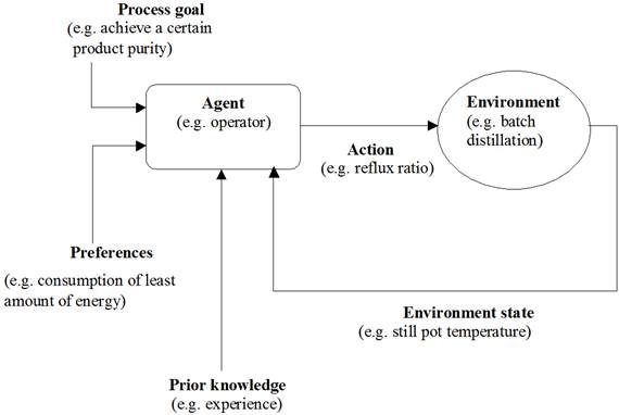
Figure 1. Main framework of Reinforcement Learning.

The Reinforcement Learning algorithm proposed by Martinez et al. [24, 25, 28] contains the following components:

a.  Value Function

Is defined as Q(s,a) which acts as the objective function, reflecting how good or bad it is to be at a certain state 襰 and taking a given action 襛

b.  Bellman Optimality Equations

The Bellman Optimality Equations form the second key component in Reinforcement Learning. In fact, by solving the Bellman Optimality Equations, the Reinforcement Learning optimization problem is solved and the optimum Value Function is calculated. One of the main advantages of Dynamic Programming [29] over almost all other existent computational methods, and especially classical optimization methods, is that Dynamic Programming determines absolute (global) maxima or minima rather than relative (local) optima [27]. Hence we need not concern ourselves with the vexing problem of local maxima and minima.

c.   Neural Network

Artificial Neural Networks take their name from the networks of nerve cells in the brain. They are computational methods, which try to simulate the learning process that takes place in the mind. The Artificial Neural Networks, usually referred to as Neural Networks (NN), learn the relationship between inputs and outputs of a function [30]. One of the widely used algorithms in NN training is the error back-propagation algorithm. One neural network is used throughout the methodology as the learning function part of the Wire Fitting approximation. Learning is achieved by adjusting the weights and biases in the NN so as to obtain better approximation to the Value Function. The NN was set in the current application as follows: 2 inputs, 1 hidden layer, 1 output and a Tansigmoidal function as the activation function.

d.  Wire Fitting

Wire Fitting [31] is a function approximation method, which is specifically designed for self-learning control problems where simultaneous learning and fitting of a function takes place. It is particularly useful to Reinforcement Learning systems, due to the following reasons: It provides a way for approximating the Value Function; It allows the maximum value function to be calculated quickly and easily (hence allowing the identification of the best action at a given state). Wire Fitting is an efficient way of representing a function since it fits surfaces using wires as shown in Figure 2. Three wires are used to support the approximation of the Value Function for all later case studies. The Interpolated Function is then defined by a weighted-nearest-neighbor interpolation of the control points as follows:

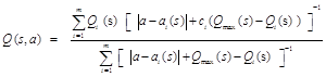  (1)

Where the constant c determines the amount of smoothing for the approximation and m defines the number of control wires.

e.   Predictive Models

Predictive models are used at each stage, instead of the actual model, to provide a one step-ahead prediction of states and reward given current state and action. The general structure of the predictive models for the various stages is provided by Eq. 2. The predictive models are as follows:

                                 (2)

where s_t+1 (state at time t+1) is a function of the current state s_t (state at time t) given a certain action a_t (action taken at time t).

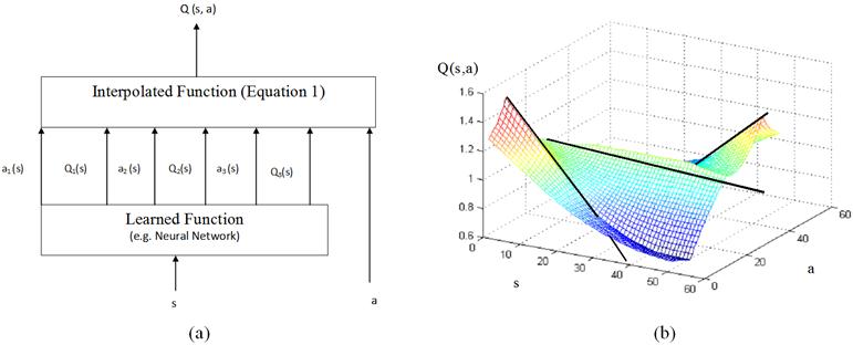
Figure 2. (a) Wire Fitting Architecture (b) Wire Fitting using 3 wires.

The criteria used for convergence, is the Bellman Optimality Equation, (Equation 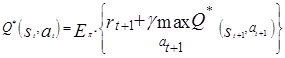3).

    (3)

where (r_t) is the reward for given a t time t.

Since the rewards (r_t) are not known, in advance, until the run has been completed, "r (s _t, a) = 0, t < T was imposed. Also, g is set to 1, since the problem breaks down into episodes. Hence, the Bellman Optimality Equation could be rewritten as follows:

                                                               (4)

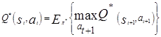
The Value Function is calculated in general using the following relationships:

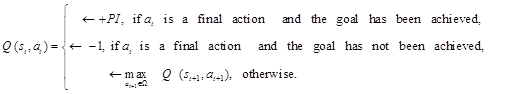               (5)

where PI is the Performance Index (a function of the final conditions at time T). Penalty of -1 is nominal value and it may be appropriate to use other values in particular problems

Since the main aim of the algorithm is defining the optimal actions which result in the optimal value function, Equation 5 could be rewritten as follows (Since the goal is always achieved with an optimal policy (*) and hence the Value Function never equals -1):

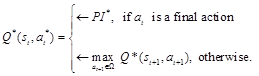                                                    (6)

Equation 6 is true only when the RL algorithm converges to the actual optimal value function. During incremental learning of the optimal value function, differences occur which define the error: Bellman error. The mean squared Bellman error, E_B, is then used in the approach to drive the learning process to the true optimal value function (Equation 7 defines E_B for a given state-action pair (s_t,a_t)).

                              (7)

The main aim of the Reinforcement Learning algorithm is to optimize the operation of the process through the following control law:

where W represents the set of feasible control actions.

                         (8)

An initial training data set is provided and the Reinforcement Learning algorithm (Figure 3) is executed offline. Following the completion of the learning phase, the Reinforcement Learning algorithm is implemented online. The control policy is then to calculate the optimal action a*, for every state encountered during progress of the batch run, based on a constrained optimization of equation 8. At the end of the batch run, the training data set is updated, followed by update of the predictive models and testing of convergence criteria..

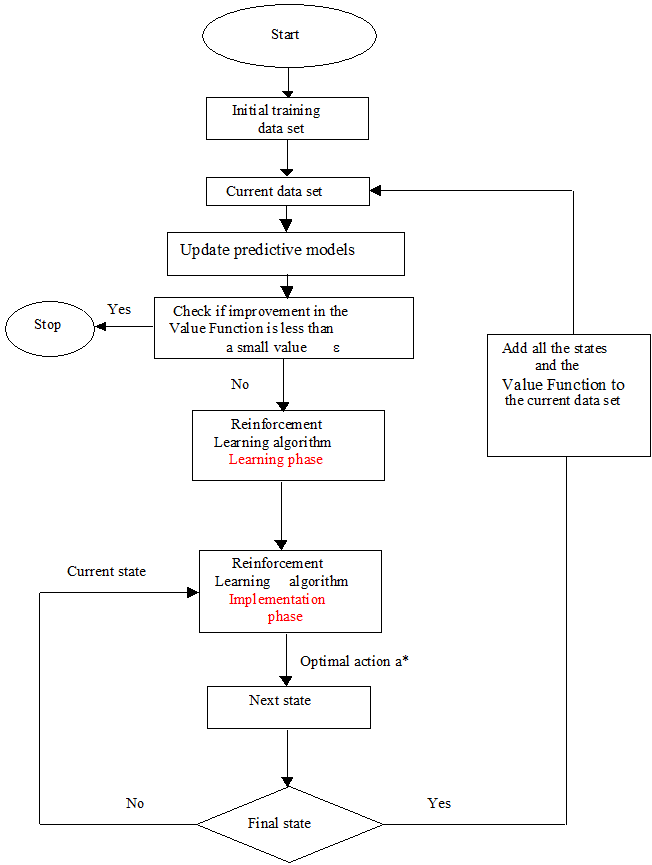
Figure 3. Summary of Reinforcement Learning algorithm.

3.1. Case Study

The RL technique is applied to a batch distillation case study which involves a 10-tray batch distillation column with a binary mixture having a relative volatility of 2.5. Simulations of the batch distillation column were conducted using Smoker's equation [32] for a binary mixture. Smoker誷 equation, although does not consider column holdup, is useful for preliminary evaluation studies, optimization problems, process control studies and real-time control algorithms [33, 34]. The operation of the batch distillation column is divided into a three-stage problem (Figure 4). The process starts at state S_T-3, corresponding to the initial state, and terminates at state S_T (at time interval T). During different time intervals (T-3, T-2 and T-1), samples of the state of the process are taken, and accordingly 3 actions are chosen (a_T-3, a_T-2, and a_T-1). States are, for example, the bubble point temperature except for the final state where it represents the product purity whereas the actions are the reflux ratios.

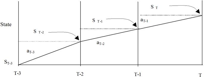
Figure 4. Three decision steps (batch distillation case study).

The strategy for operating and simulating the batch distillation column was set as follows:

1.  The still is initially charged with a feed of 1 kmol containing 0.7 mole fraction of the more volatile component. The specification for the product purity was set at 0.98 mole fraction.

2.  Three periods of operation each at a fixed reflux ratio (i.e. three decision steps as shown in Figure 4).

3.  Still temperature measured and used to decide on change to reflux ratio when still pot contents lie at 1.0, 0.68 and 0.48 kmol (those values were selected following an analysis of optimal operation of case study). The temperatures were calculated using the following relationship [33]

TS = ((17.7507x-17.2679)x-30.5983)x+109.7767    (9)

where TS is the temperature of the still pot and x is the mole fraction of the more volatile component in the still

4.  Each batch is terminated when still pot contents falls to 0.35 kmol.

5.  Constant vapour boilup rate of 0.2 kmol/h.

6.   The target for the RL algorithm is then set to achieve the goal of obtaining a product purity of 0.98 mole fraction. In addition, the preference is given to meeting the goal in the minimum amount of time so as to achieve the maximum profit. The Performance Index (PI) is defined as follows:

PI = D. P_r V. BxTime.C_s                  (10)

where D is the amount of product distilled (kmol), P_r is the sales value of product (kmol), V is the vapour boilup rate (kmol/h), BxTime is the time for completion of batch and C_s is the heating cost kmol.

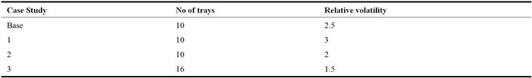
Three additional case studies, with the same feed and product specifications as in base case, were investigated with feed mixtures having different relative volatilities and numbers of column trays (Table 1).

Table 1. Description of various case studies.

A comparison between the different case studies is possible through the measure defined by Kerkhof and Vissers [14], s_diff, which indicates the degree of difficulty of separation:

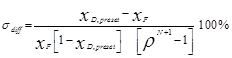      (11)

where x_D,preset is the pre-set product purity (mole fraction), x_F is the feed purity (mole fraction), r is the relative volatility and N is the number of theoretical plates in the column. They further categorize the results into the following: Easy separation (s_diff <1%), Moderate separation (1%< s_diff <10%), Difficult separation (s_diff >10%) and very difficult separation (s_diff >15%). Hence, according to those categories, base case (s_diff = 0.08%), Case study 1 (s_diff = 0.01%), Case study 2 (s_diff = 0.98%) and Case Study 3 (s_diff = 2.03%) represent easy to moderate degrees of difficulty of separation. The predictive model for the last decision stage at T-1 is

                            (12)

for the intermediate decision stage at T-2

                              (13)

where s_t (state at time t) denotes the bubble point temperature of the mixture in the still pot (representing the composition of the mixture), with the exception of the last decision stage T-1 where it represents the final product purity (mole fraction), and a_t (action taken at time t) denotes the reflux ratio.

For the initial stage there is a slight difference in the predictive model, since all batches were assumed to start from the same initial point. This would mean that the predictive model would have no dependency on the initial state, and hence the state at T-2 (still pot temperature at T-2) becomes only a function of the action at T-3 (reflux ratio at time T-3).

3.2. Development of Predictive Model

Observing the behaviour of a distillation column (i.e. separate from RL) for the various case studies, would allow a regressive model form to be chosen to capture relationships between variables of interest. Starting from different initial states (still pot temperatures), and applying a range of actions (reflux ratio's), the resulting states (still pot temperatures or product purity for last but one stage) were calculated for the various case studies as shown in Figure 5 to 7. Similar trends of lines curving initially and then gradually reaching asymptotic values is observed for all case studies.

Figure 8 shows the final product purity as a function of still pot temperature at T-1 (lines of constant reflux ratio) for the distillation column in base case. Figure 9 shows the still pot temperature at T-1 as a function of the still pot temperature at T-2 at lines of constant reflux ratio for base case. Linear and approximately parallel lines can be observed at both stages. The initial stage (T-3 to T-2) was not investigated since it is assumed that the predictive model starts from the same initial staring point (for each specific case study) and thus was a function of reflux ratio only. Similar relationships were observed for all other case studies.

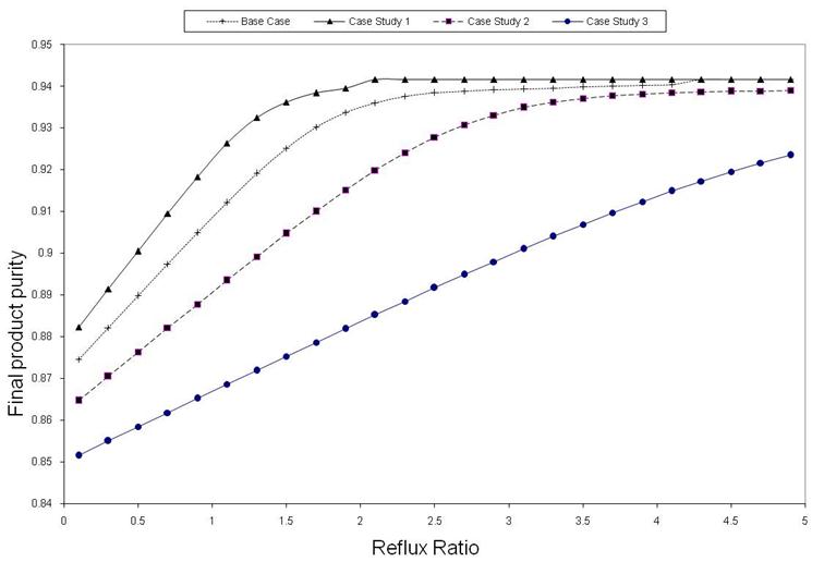
Figure 5. Final product purity as a function of reflux ratio at T-1 (Fixed still pot temperature at T-1) for the various case studies.

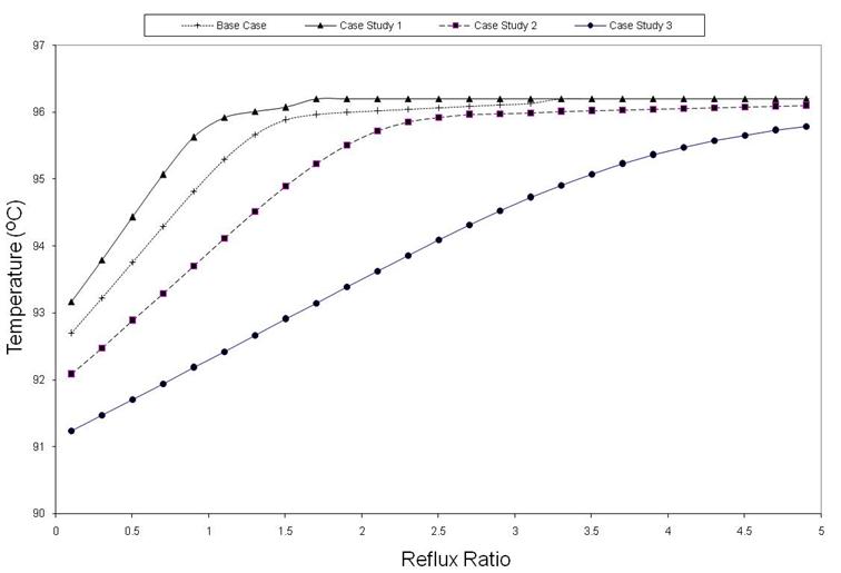
Figure 6. Temperature at Stage T-1 as a function of reflux ratio at T-2 (Fixed still pot temperature at T-2) for the various case studies.

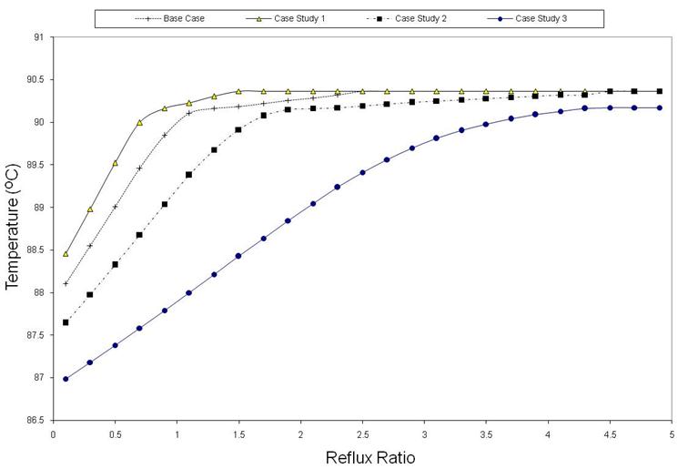
Figure 7. Temperature at Stage T-2 as a function of reflux ratio at T-3 (fixed still pot temperature at T-3) for the various case studies.

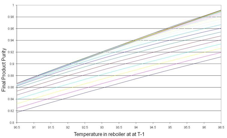
Figure 8. Final product purity as a function of still pot temperature at T-1 (lines of constant reflux ratio) for the base case.

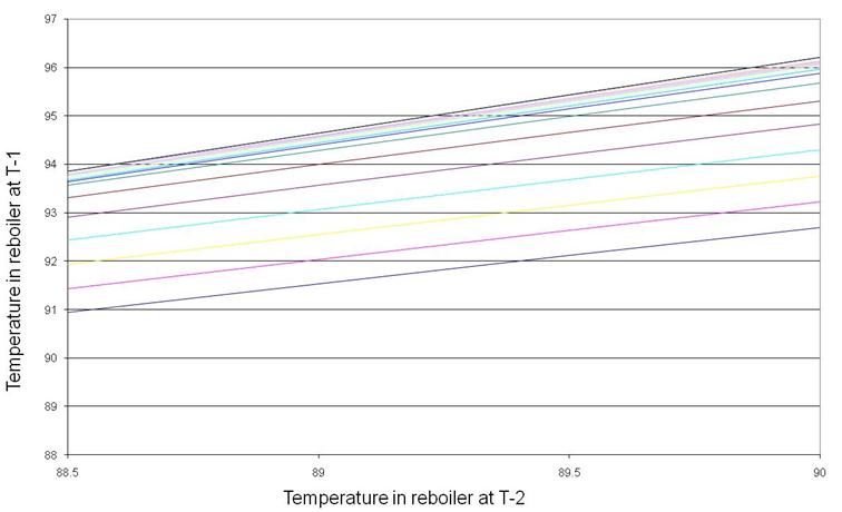
Figure 9. Still pot temperature at T-1 as a function of still pot temperature at T-2 (lines of constant reflux ratio) for the distillation column in base case.

The use of a simple predictive model (Table 2) was investigated to capture the trends presented in Figure 5 to 9. Figure 10 shows how the model seems to adequately capture the trends for the base case (Relative volatility =3) and Case Study 3 (Relative volatility =1.5) especially for intermediate values of reflux ratios.

Table 2. Description of proposed predictive model forms for different stages where s is state (temperature or final product purity composition) and a is action (reflux ratio).

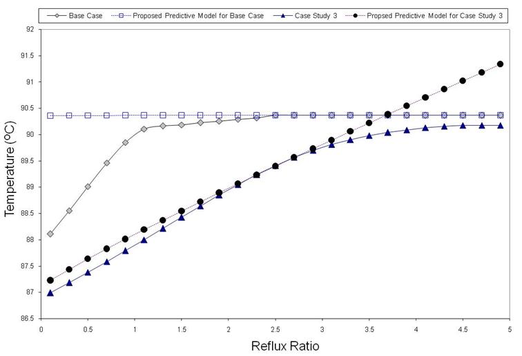
Figure 10. Use of Model S for base case and case study 3 at stage T-1 to T to fit the relationship between final product purity as a function of reflux ratio at T-1 (dotted lines represent predictions of Model S).

4. Results and Discussion

Starting with an initial training data set of six batch runs, the RL algorithm with an embedded predictive model (Q-S-S) was applied using MATLAB. The values of all free parameters (α, b and p) in the predictive mode are computed based on a constrained optimization MATLAB routine so as to provide a best fit with the current training data set. To investigate the minimum amount of batches required for learning, the RL algorithm was repeated twice using the same initial training data set equally split into 2 sets of three batch runs. The RL algorithm was executed, for all cases, until a total number of 24 batch runs were produced (including the initial training data set). The results obtained are shown in Figure 11 and clearly demonstrate how the RL algorithm has managed to incrementally improve beyond the best performance achieved in the initial training data set of 40.9 to achieve a Performance Index of 44.22 in Run 3.

The next step was to apply the RL algorithm to case Study 1 (α=3 and number of trays = 10) using 3 sets of initial training data. The first set consists of 6 batches whereas the two other sets consist of the same 6 batches equally split into 2 sets. The results obtained are shown in Figure 12 and clearly demonstrate how the RL algorithm has successfully managed to incrementally improve beyond the best performance achieved in the initial training data set of 47.4 to reach a new value of 49.37.

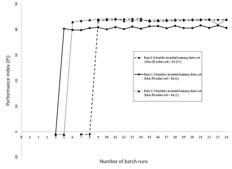
Figure 11. Performance Index as a function of number of additional batch runs (using one set of 6 initial batch runs and 2 sets of 3 batch runs each) for base case.

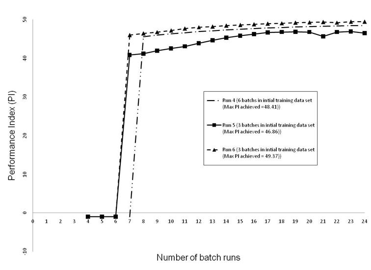
Figure 12. Performance Index as a function of number of additional batch runs (using one set of 6 initial batch runs and 2 sets of 3 batch runs each) for Case Study 1.

The results shown on Figure 11 and 12 reveal how sometimes no off-spec batches (Figure 11, Run 2), 1 off-spec batch (Figure 11, Run 1 and 3) or even 3 off-spec batch runs are produced (Figure 12, Run 5 & 6) before actual improvement in PI takes place. The results produced, through the application of the RL algorithm, seem to be dependent on the quantity and quality of the initial training data set provided for learning.

The RL algorithm was further applied to case Study 2 (α=2 and number of trays = 10) using 3 sets of initial training data. The first set consists of 6 batches whereas the other two sets consist of the same 6 batches equally split into 2 sets. The Results obtained are shown in Figure 13. It is clear that although there is a steady improvement in PI, however using the 6 batch initial data set (Run 7) results in the production of off-spec batches (PI=-1). Runs 8 and 9 produce a steady, although small, improvement in performance which is clearly related to the higher degrees of difficulty of separation.

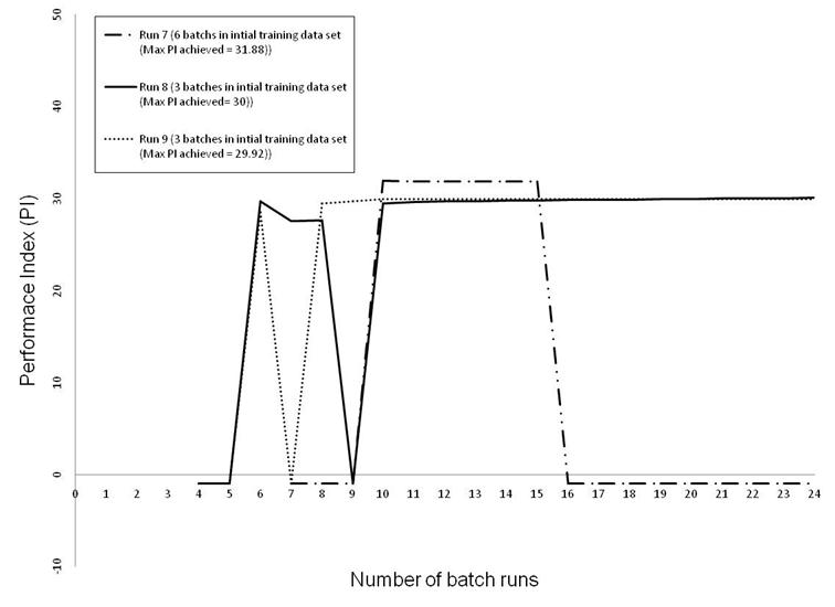
Figure 13. Performance Index as a function of number of additional batch runs (using one set of 6 initial batch runs and 2 sets of 3 batch runs each) for Case Study 2.

Give-away is a common term in industry and is used when dealing with problems where a hard constraint has to be met and could not be violated. For example the goal, in the case studies presented, is to meet a product purity of 0.98 mole fraction. If the batch distillation is controlled in practice along that value of product purity, the controller is bound to produce off-spec batch runs some of the time. Hence in industry, they are willing to give away a slightly more pure product on average, so as to reduce the risk of losing money through production of off-spec batches. Hence, the term give-away in this context refers to the amount of average product purity that one could give-away above the fixed product specification. Concerning the analysis in the following sections, the product specification is set throughout at 0.98 mole fraction. Give-away values of 0.005 are used to reflect how all batches produced to a product purity of 0.975 fraction is accepted as being on-spec. The RL algorithm was again repeated for the failed run (6 batches in initial training data set) with a giveaway in product purity of 0.005. It is clear that the RL algorithm has steadily managed to improve the PI and to produce additional batches with product purity above 0.975 except in an odd case where an off-spec batch is produced (Figure 14). This shows that although off sepc batches are produced, this happens due to a very small violation of the product purity specs.

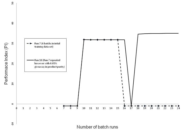
Figure 14. Performance Index as a function of number of additional batch runs (using same set of 6 initial batch runs however with and without a giveaway in product purity of 0.005) for Case Study 2.

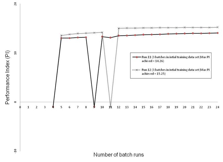
Figure 15. Performance Index as a function of number of additional batch runs (best batch run in initial training data set results in a PI equal to 11.36) for Case Study 3.

The RL applications to case study 3, using 2 sets of 3 initial training batch runs, produced only off-spec additional batches (i.e. which did not meet the goal). The RL algorithm was thus repeated using the same initial training data set of 3 batches however with 0.005 give away in product purity. The RL algorithm successfully managed to improve the PI value and to produce on-spec batches as shown in Figure 15. It is evident that the main challenge with such kind of optimization problems is that a hard constraint needs to be met. PI values of -1 do not necessarily mean that the batches produced are widely off-spec as values of product purity slight less than 0.98 are considered off-spec. This is clear when giveaway values of 0.005 in product purity are allowed; all subsequent produced batch runs are on-spec. Thus it is clear that it is crucial, for further applications of the RL algorithm, to allow for a slight giveaway in product purity to avoid production of off-spec batches. Furthermore, there is a trade-off between the learning rate of the RL algorithm (exploration of new state-action pairs) versus the possibility of losing performance through the production of off-spec batch runs. A less aggressive exploitation of the existing accumulated data will guarantee that no off-spec batches are produced however at the expense of very slow convergence of the RL algorithm (Lots of additional batch runs may be required to reach near optimal PI values).

4.1. Introduction of Process Uncertainty

One of the issues facing the methodology in real practice would be the issue of random disturbances or uncertainty in process states. Uncertainty was simulated by the addition of random noise to the value of intermediate states (random noise was added to states at T-2 and T-1 for the initial training data set and for all subsequent intermediate states. Final product purity measurements were assumed to be unaffected) representing, for example, errors in measurements or sampling. To achieve this, a random number generator was used to generate random numbers with mean zero and variance one. Three runs were produced using 10%, 50% and 100% respectively of random disturbances produced through the MATLAB function 襌ANDN In each case the random number generator was initially reset to the same state.

Incremental learning of the Value Function was conducted for cases study 3 (moderate degree of difficulty of separation [14] using three levels of noise and an initial training data set of 3 batches. The results for the three runs (Figure 16) show the effect of disturbances on the performance of the Reinforcement Learning algorithm, and the speed of convergence. As the disturbances increase, the performance becomes worse and the algorithm takes longer to learn the optimal profile. This is in agreement with what might be expected with high noise levels. On the other hand, fairly similar trends are followed in the three cases, which show that the Reinforcement Learning algorithm is able to cater for uncertainties in process states.

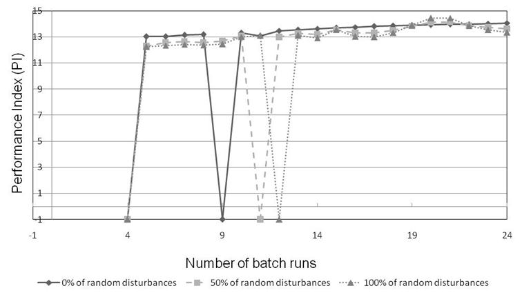
Figure 16. Effect of introducing uncertainty in process measured states on incremental learning of value function for Case Study 3.

4.2. Conclusions

Reinforcement Learning application has shown huge potential and a step towards full automation of batch distillation. Following the analysis of data from different case studies, a predictive model has being put forward. It is demonstrated how predictive model Q-S-S is able to adequately capture the different trends for the various case studies. The results obtained are quite impressive if taken into account that the algorithm has learned the Value Function without knowledge of VLE data and with a minimum initial training data set of three batch runs. The RL algorithm produces very encouraging results for easy separations as defined by Kerkhof and Vissers [14]. For moderate separation, smaller improvements in Performance Index are produced, however slight giveaway in product purity is required to make sure that production of off-spec batches is reduced. Furthermore, it was shown that the introduction of random process disturbances degrades the performance of incremental learning, as expected, however similar trends are maintained with different levels of noise. Thus, the Reinforcement Learning algorithm is shown to be able to deal with practical issues regarding uncertainty.

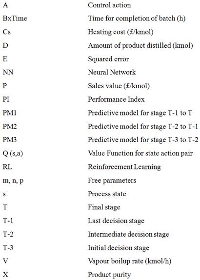
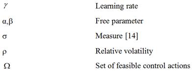
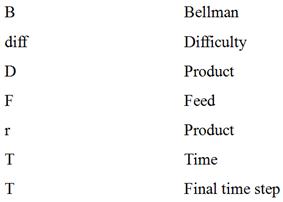
Nomenclature

Greek Letters

Subscripts

Superscripts

References

1. Diwekar U. M. Batch distillation: Simulation, optimal design and control. Carneige Mellon University, Pittsburg, Pennsylvania; 1995.
2. Luyben W. L. Practical Distillation Control. Van Nostrand Reinhold. New York; 1992.
3. Bonny L., Domenech S., Floquet P., Pibouleau L. Recycling of slop cuts in multicomponent batch distillation. Comput. Chem. Eng. 1994; 18: S75-S79.
4. Mujtaba I. M. and Macchietto S. An optimal recycle policy for multicomponent batch distillation. Comput. Chem. Eng. 1992; 16: S273-S280.
5. Sorensen E. Alternative ways of operating a batch distillation column. Institution of Chemical Engineers Symposium Series 1997; 142: 643-652.
6. Farhat S., Czernicki M., Pibouleau L., Domenech S. Optimization of multiple-fraction batch distillation by nonlinear programming. AIChE Journal 1990; 36: 1349-1360.
7. Converse A. O., Gross G. D. Optimal distillate-rate policy in batch distillation. Ind. Eng. Chem. Fund. 1963; 2: 217-221.
8. Keith F. M., Brunet. Optimal operation of a batch packed distillation column. Canadian J. Chem. Eng. 1971; 49: 291-294.
9. Coward I. The time optimal problem in binary batch distillation. Chem. Eng. Sci. 1967; 22: 503-516.
10. Mayur D. N., Jackson R. Time optimal problems in batch distillation for multicomponent mixtures columns with hold-up. Chem. Eng. J. 1971; 2: 150-163.
11. Egly H., Ruby N., Seid B. Optimum design and operation of batch rectification accompanied by chemical reaction. Comput. Chem. Eng. 1979; 3: 169-174.
12. Hansen T. T., Jorgensen S. B. Optimal control of binary batch distillation in tray or packed columns. Chem. Eng. J. 1986; 33: 151-155.
13. Mujtaba I. M., Hussain M. A. Optimal operation of dynamic processes under process-model mismatches: Application to batch distillation. Comput. Chem. Eng. 1998; 22: S621-S624.
14. Kerhof L. H., Vissers H. J. M. On the profit of optimum control in batch distillation. Chem. Eng. Sci. 1978; 33: 961-970.
15. Logsdon J. S., Diwekar U. M., Biegler L. T. On the simultaneous optimal design and operation of batch distillation columns. Chem. Engi. Res. Des. 1990; 68: 434-444.
16. Mujtaba I. M., Macchietto S. Efficient optimization of batch distillation with chemical reaction using polynomial curve fitting. Ind. Eng. Chem. Res. 1997; 36: 2287-2295.
17. Cressy D. C., Nabney I. T., Simper A. M. Neural control of a batch distillation. Neural Computing and Applications 1993; 1: 115-123.
18. Stenz R., Kuhn U. Automation of a batch distillation column using fuzzy and conventional control. IEEE Transactions on Control Systems Technology 1995; 3: 171-176.
19. Wilson J. A., Martinez E. C. Neuro-fuzzy modeling and control of a batch process involving simultaneous reaction and distillation. Comput. Chem. Eng. 1997; 21: S1233-S12.
20. Barolo M., Cengio P. D. Closed-loop optimal operation of batch distillation columns. Comput. Chem. Eng. 2001; 25: 561-569.
21. Kim Y. H. Optimal design and operation of a multi-product batch distillation column using dynamic model. Chem. Eng. Process. 1999; 38: 61-72.
22. Lopes M. M., Song T. W. Batch distillation: Better at constant or variable reflux? Chem. Eng. Process: Process Intensification 2010; 49: 1298-1304.
23. Pommier S., Massebeuf S., Kotai B., Lang P., Baudouin P., Floquet P., Gerbaud V. Heterogeneous batch distillation processes: Real system optimization. Chem. Eng. Process: Process Intensification 2008; 48: 408-419.
24. Martinez E. C., Pulley R. A., Wilson J. A. Learning to control the performance of batch processes. Chem. Eng. Res. Des. 1998a; 76: 711-722.
25. Martinez E. C., Wilson J. A. A hybrid neural network first principles approach to batch unit optimization. Comput. Chem. Eng. 1998b; 22: S893-S896.
26. Mustafa M. A., Wilson J. A. Application of Reinforcement Learning to Batch Distillation, The Sixth Jordan International Chemical Engineering Conference, 12-14 March 2012, Amman, Jordan, 117-126.
27. Sutton R. S., Barto A. G. Reinforcement Learning: An Introduction, The MIT Press, Cambridge, Massachusetts, London, UK; 1998.
28. Martinez E. C., Wilson J. A., Mustafa M. A. An incremental learning approach to batch unit optimization. The 1998 IChemE Research Event, Newcastle; 1998c.
29. Bellman R. Dynamic Programming, Princeton University, Press, Princeton, New Jersey; 1957.
30. Carling A. Introducing Neural Networks, SIGMA Press, UK; 1992.
31. Baird L. C., Klopf A. H. Reinforcement Learning with High-dimensional Continuous Actions, Technical Report WL-TR-93-1147, Wright Laboratory, Wright Patterson Air Force Base; 1993.
32. Smoker E. H. Analytical determination of plates in fractionating columns. Trans AICHE 1938; 34: 165.
33. Tolliver T. L., Waggoner R. C. Approximate solutions for distillation rating and operating problems using the smoker equations. Ind. Eng. Chem. Fundam 1982; 21: 422-427.
34. Jafarey A., Douglas J. A. McAvoy T. J. Short-Cut Techniques for Distillation Column Design and Control. 1. Column Design. Ind. Eng. Chem. Process Des. Dev. 1979; 18; 2: 19702.