An Interactive Simulation of the Cardiomyocyte Cycle for Medical Education

Lazaros Papadopoulos^{1, *}, Eva Comaroski²

¹Laboratory of Medical Informatics, Medical School, Aristotle University of Thessaloniki, Thessaloniki, Greece

²Department of Computer Science, Birmingham University, Birmingham, UK

Abstract

In early medical education, myocardial electrical behavior is taught by studying the Action Potential (AP) phases and membrane ionic currents. Cellular automata theory can be used to create educational simulations. The aim of this paper was to develop a cardiac electrical activity e-learning tool in Second Life. Myocardial tissue is represented by a network of primitives each having the option of being a stimulus generator. A cell broadcasts messages across the network during depolarization. When a broadcast is received by a neighboring cell, the distance is calculated and compared to a threshold, so that cells cannot get activated by distant neighbors. Electrical propagation is simulated with the use of a probabilistic model of diffusion. The spread of the stimulus is visualized by assigning a color for each AP phase. The simulation is created using the Linden Scripting Language and allows the user build cellular boards create pulse generators or necrotic cells and adjust AP timing, providing the ability to create visualizations of normal myocardial electrical activity, thus promoting e-learning processes through constructivism. Pathological circuits such as reentrance are also simulated.

Keywords

Medical Education, Simulation, Second Life, Cellular Automata, Virtual World, Electrophysiology, Heart

Received:July 20, 2016
Accepted: August 3, 2016
Published online: August 19, 2016

@ 2016 The Authors. Published by American Institute of Science. This Open Access article is under the CC BY license. http://creativecommons.org/licenses/by/4.0/

1. Introduction

Established teaching practices in electrophysiology include class-based lectures, demonstrations in the lab and studying textbooks. The difficulty of teaching excitable tissue’s properties arises from the fact that a visual observation of the electrical effects is not possible. As a consequence, undergraduate students rely on the book’s illustrations and their imagination in order to understand the propagation of an electrical stimulus across a row of connected excitable cells. Imperfect comprehension of these concepts leads to misconceptions that teaching methods may fail to alleviate [1]. Simulation can assist educators in explaining these phenomena and offer learning experiences. Within a simulated environment students can observe, repeat and alter the parameters of a process, without cost or hazard. Simulation is widely used in health education in order to improve trainees’ performance and allow them to apply their theoretical knowledge in a safe environment [2,3].

The first mathematical model of ionic behavior in excitable tissues was described by Hodgkin and Huxley (HH) in 1952, according to which each of the ionic currents is described as a multiplication of the ion’s conductance by the corresponding transmembrane potential [4]. The activation and inactivation of ion channels are described through differential equations and so, the describing system is nonlinear. Many other models based on the HH model have been developed (reaction-diffusion systems), involving multiple state variables to describe the action potential (AP) [5,6,7,8]. These models are considered accurate but they are also characterized by a great level of detail and complexity. Thus, the simulation of the electrical activity of even a piece of cardiac tissue, based on a reaction-diffusion system, requires high computational resources and complex programmable techniques as illustrated by Chorro Gascó [9]. Using these models in order to build an educational simulation may be impractical.

Another way of mathematically describing an excitable tissue's activity is by using cellular automata; each cell is considered to be an automaton with a finite number of states. The transitions between the states are governed by rules based on the cardiac cell’s AP concepts. Simulation of excitable tissues with cellular automata has been described by using various models of diffusion [10,11,12,13,14]. One recent and promising technique, aiming to reduce the complexity of reaction-diffusion systems while incorporating the simplicity of the automata theory, is the Hybrid Automata (HA) [15]. Bartocci et al have developed CellExcite, a computer simulation environment for excitable cell networks based on HA [16]. Atienza et al [14] and recently, Khan et al [17] have depicted the states of the cardiac cells cycle using automata. Balakrishnan et al proposed a computational 2D whole heart model to explain many types of arrhythmias in relation to electrocardiogram signal [18]. We believe that cellular automata can be widely used in order to create simple but yet descriptive simulations of the electrical propagation in the heart for use in undergraduate level.

When designing educational software, one must make decisions about the programming language, the user interface design and the distribution of the software. Virtual Worlds (VWs) offer a plethora of tools for building an educational application. A VW is a synchronous and persistent network of people, represented as avatars, facilitated by networked computers [19]. This world contains a persistent online social space, a virtual environment that people experience as ongoing over time and that have large populations which they experience together with others as a world for social interaction [20]. Medicine has found its place in this virtual world. In particular, SL currently hosts a number of medical and biology education projects. For example, the Genome Island in SL offers a 3D tour inside a cell and its organelles [21]. The Anatomica of the American Cancer Society [22] is an e-learning environment in SL that enables visitors to examine the functions of the immune system and visualize the white cells. Various types of hospital rooms including emergency, intensive care and others can be found at Evergreen Island [23]. In the Ohio State University Medical Centre in SL [24] the students can examine 3D models of human testis and ovary and walk inside the organs to develop a better understanding of their design and function. VWs also show great potential in teaching aspects of pediatric dentistry, with the use of a virtual patient in a virtual dental clinic [25]. SL’s potential in medical educational applications has been described in recent reports [26,27]. Conradi et al created five virtual patient scenarios in SL; student’s feedback showed an effective engagement in learning, better than classroom based scenarios [27]. In general, virtual worlds are believed to have a great potential as learning environments, because they offer opportunities for simulations, role playing, interactions, and constructivism while the virtual co-presence encourages sociability and motivates students to engage and attend [28].

In this paper we present the principles for developing an e-learning tool for simulating myocardial cells’ activity in Second Life. The Cardiac Electrical Activity Simulator (CEAS) combines cellular automata with a probabilistic diffusion model. In the Methods section we describe the mathematical and programming background of CEAS, while in the Results we demonstrate its features and capabilities.

2. Methods

The heart contains different kinds of cells that generate, conduct and respond to electrical impulses. The myocardial cells propagate the electrical stimulus as a specific type of electrical pulse, the AP. The AP is a short electrical event during which, each cell’s membrane potential rapidly rises and then falls, forming a typical pattern. Its curve consists of 5 phases (Figure 1). The fast voltage gated Na⁺ channels permit rapid influx of sodium ions at the beginning of the AP (phase 0 or depolarization phase). This is caused by the transmission of stimuli from the surrounding cells and alters the membrane potential from -90mVolts to approximately +50mVolts. The inactivation of these channels leads to the next, short, phase 1. The "plateau" or phase 2 is the result of Ca⁺² inward and K⁺ outward movements through the membrane's potassium and L-type calcium channels. This phase prolongs the AP duration on purpose; the first stimulated cells of the myocardium are still in refractory state when the AP reaches the last cells of the myocardium. This prevents cyclic re-entries of APs. Phase 3 (repolarization phase) occurs when K⁺ outward increases and Ca⁺² channels are deactivated. This leads membrane back to its resting potential (phase 4). The duration of ventricular AP ranges from 200 to 400 milliseconds [29,30]. Abnormal behavior of the ion channels, disturbances in the propagation among the cells or impulses originating from ectopic focuses lead to arrhythmias [18,31].

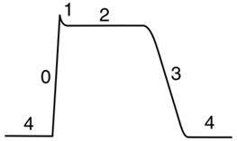
Fig. 1. The Action Potential of a myocardial cell.

2.1. Overview of the Probabilistic Model of Diffusion

The probabilistic model of diffusion presented by Atienza et al describes the electrical propagation based on probabilistic parameters [14]. Our paper utilizes the probabilistic model of diffusion. A cell is represented by a deterministic finite automaton (DFA) with three states: resting, refractory 1 and refractory 2. When a cell is in the refractory 1 state, it stimulates its adjacent cells. The transmission of the stimulus to these cells and therefore, the whole propagation, is assumed to be probabilistic according to the authors. The probability that one cell will be depolarized, or in other words, the transition from phase 4 to phase 0 of the AP, is calculated using the following formula:

                          (1)

Where E represents the cell’s excitability level which increases in time, A is the binary excitation state of the cell i (1 if refractory, 0 if not), the distance between the cell at index i and the cell at index j with the extra condition that i≠j, Pj denotes the probability that cell j is excited [14].

2.2. Cell Network

In order to simulate a cell-network, we make use of LSL’s API function llMessageLinked to broadcast messages across a set of linked objects in SL, called primitives.

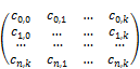
A cell-network is thus, in our abstraction, given by an unbalanced matrix of elements:

                 (2)

where every cell c1,…,cn is a linked primitive in the link-set, containing a DFA. The columns of matrix CN give us the height of the matrix and the rows give us the length of the matrix. Geometrically, this reduces the model to one layer of cells where the messages are propagated across an x,y-plane (Figure 2). This is similar to what Atienza et al define as: d(i,j), the distance between the cell at index i and the cell at index j with the extra condition that i≠j. This is because the distance between a cell and itself is 0, which would result in division by zero. In terms of our simulator, the i≠j condition is satisfied by disallowing cells to listen to their own messages. The simulator uses both E and A implicitly such that every time a message is received by a cell, the probability for that cell to commute to refractory 1 increases.

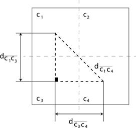
Fig. 2. Every cell of the matrix can be projected on a plane in order to calculate the relative distances to all neighboring cells.

2.3. Distance Calculations on the Cell Network

Given a general matrix CN (Cell Network) with n rows and k columns:

                         (3)

and knowing that the cell-number is bounded such that:

We take the distance between the adjacent elements to be 1 unit, which allows us to determine the series via geometric induction over the triangles generated by the diagonal of the matrix CN.

In the base case for i=0 and j=0, for the triangle  in Figure 2 we know that both sides are equal given the 1 unit diameter of each cell. Thus, we obtain that:

                      (4)

and by applying Pythagoras in , we obtain that:

                   (5)

Now, we extend the triangle further, increasing each side by 1 unit so that i→i+1 and j→j+1 obtaining thus a larger triangle described by the cells.

From (1), we obtain that the length of the segments is now:

                   (6)

and by applying Pythagoras again in the extended triangle given by the cells , we obtain that:

                 (7)

and by substituting from (2), we obtain that:

                 (8)

Finally, let that i→n and that j→n and following the induction over triangles, we obtain a generalized triangle given by the cells . By applying Pythagoras again, we obtain the distance:

                      (9)

Substituting the distance into formula (1) we obtain the probability for a cell to activate relative to the distance to the neighboring cells on the entire cell matrix:

                    (10)

We can illustrate the activation heat-map based on distances relative to a cell waiting to be activated can be seen from Figure 3.

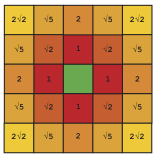
Fig. 3. Each red cell is labeled with the distance relative to the green cell in the middle that receives activation messages. The probability to activate the middle is directly proportional to the distance from the 24 neighboring cells. The colored shading from red to yellow illustrates the influence that the cells have on the green cell to be activated.

2.4. Myocardial Automaton

The DFA that we use for the CEAS is based on four main states and three auxiliary states which allow the user to control the simulation. In the final extended model, we split refractory 2 into refractory 2a and refractory 2b in order to simulate the plateau (phase 2) and rapid repolarization (phase 3).

One of the features of the LSL language is that it exposes the concept of states on the upper layers of the language semantics. We are able to explicitly define and observe states as being a construct within the syntax of the language itself. Each state in LSL marks an untyped label, referencing a set of event callbacks that run locally to that state. In LSL every state may subscribe to global events and process them using the corresponding callbacks. Any transition from one state to the other is performed by using the state command followed by the label of the next state. This gives the language the possibility of two types of continuations [32] one in the automata context where transitions are made from state to state by using the state command and the widespread GOTO-like jumps by using the LSL jump command. Jump labels are locally scoped to the state or function where they are placed whereas state-transitions are globally scoped. One of the elegant outcomes is that we are able to model automata by reasoning about state transitions on the upper layer of the programming semantics. In Figure 4 and 5 we have sketched some crude LSL code that represents the starting framework, which was later expanded into the complete code of the CEAS. The CEAS consists of individual cells represented by objects and every object contains a seven-state DFA which is based on an extended version of the code in Figure 5.

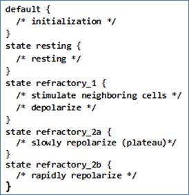
Fig. 4. Outline of the CEAS using a 4-state DFA in LSL. All the refractory states can be expressed directly in code which makes it much easier to reason about the program logic.

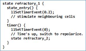
Fig. 5. Switching from the state refractory 1 to refractory 2 can be done by scheduling an event using the command llSetTimerEvent that will commute to the refractory 2 state after a specified amount of time.

The entire framework consists in an allotment of state labels which we use to model the transition between the states default, resting, refractory 1, refractory 2a and refractory 2b (Figure 6). Applied to the CEAS, the duration of the AP is by default set to 250ms. Given that every cell stimulates its neighbor during the refractory 1 state (phases 0 and 1) which represents about 10% of the whole ventricular myocyte cycle, the primitive will stay in the refractory 1 state for 20ms.

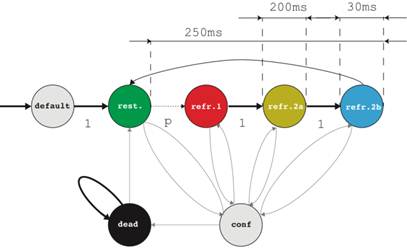
Fig. 6. Every cell contains a 4-state DFA representing the four stages of the AP. We use the default state for initialization, the configuration state to set the parameters of the simulation and an additional dead state to represent necrotic cells.

2.5. Algorithm

In order to broadcast messages, we use the function llMessageLinked across a grid of primitives. Every single primitive has an index, corresponding to the matrix of cells. Whenever a cell i,j becomes activated, that cell broadcasts a message to all the cells on the board of cells representing the tissue corresponding to the matrix CN. We add a limitation that a cell on the matrix CN will filter out any messages that are further away than two cells distance as seen in Figure 3. Thus, a cell only takes into account the messages broadcasted by the 24 cells in its vicinity and any other messages that propagate through the board are ignored. This has the consequence that direct neighboring cells will always activate a cell but the cells that are further away will only contribute a fraction of the probability required to activate the cell.

At any point, regardless of the state of the cell, the user may choose to commute to the configuration state in order to configure AP parameters of the cell. Although the model has been built using fictive time units, users may choose any real values for the simulation through the options menu. The values defined by the user are automatically multiplied by 100ms. In this way, CEAS provides not a real-time but rather a scaled or slow-motion simulation. This is done solely for educational purposes; CEAS is not an accurate research tool, but primarily an educational simulator. Individual cells also benefit from an optional dead-state which allows users to make the cells necrotic. In the necrotic state, the cell is considered dead and is not able to receive messages or commute to other states. The pseudo code of the algorithm that we use for commuting the automaton from resting to refractory 1 is shown in Figure 7. The complete code of CEAS and demonstrational videos may be found on the Grimore website [33].

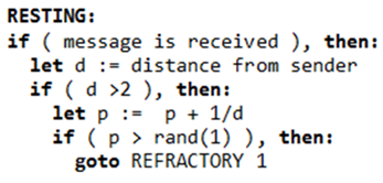
Fig. 7. Automaton transitions can be modeled by using jumps. Automaton commutes to the refractory 1 state once a cell has been influenced sufficiently by neighboring cells in order to exceed the probability threshold.

3. Results

CEAS allows users to build boards and circuits of cardiac cells in SL, change the timing of the AP phases and simulate various normal and pathological conditions, such as reentries.

3.1. Setting up CEAS – User Interface

CEAS is freely available from SL’s marketplace [34] as a cube that is deployed by a touch event. The user defines the desirable dimensions of the cellular board. Once the board is built, the cells must be manually linked to each other. Using Set phase 2 and Set phase 3 options user can define the duration of the plateau and rapid repolarization phases of the selected cell (Figures 8, 9). Every value entered is automatically multiplied by 100ms. The AP’s default values are shown in Table 1. With the Start option the selected cell start generating impulses, while with the Set Gen option the user specifies the frequency of the stimuli production. Also if the Start option is applied in a distant cell, the user can create ectopic stimuli in order to simulate abnormal conditions. The Show RP and Hide RP buttons reveal the total repolarization (RP) time of each cell on the board; this is the sum of the AP’s phase 2 and phase 3 durations. This feature is useful when designing pathways on the board across which the propagation is expected to travel faster or slower. The Kill Cell allows the user to create necrotic cells and obstacles on the board. The Reset option brings the cell back to default settings. There is also a Help button which gives the user a notecard with instructions. Finally the Fib starts an atrial fibrillation demonstration.

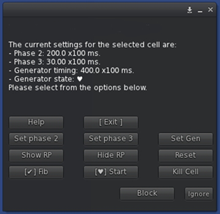
Fig. 8. Control Window.

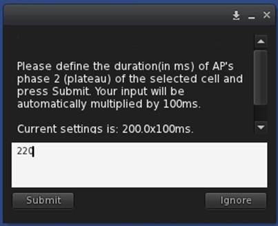
Fig. 9. Adjustments of AP phase 2 of the selected cell.

3.2. Example of a Normal Network and Propagation

In this section is presented the simulation of a normal cell network using the default AP values of CEAS. In Figure 10(A) a generator cell is set in coordinates (10, 7) of the board. Each cell changes color according to its current state. The correspondence of colors and AP phases is shown in Table 1. The propagation is illustrated in Figures 10(B to E).

Table 1. AP phases, durations and representation in CEAS.

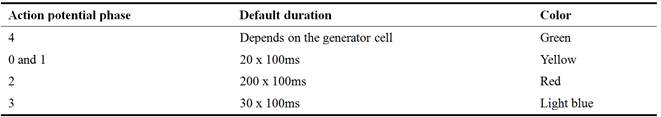
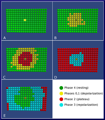
Fig. 10. A) The generator cell produces a pulse. The board is in the resting state (green). B) Cells become depolarized (yellow) as the stimulus is being transmitted from the center cells to the periphery. C) Cells in the center enter plateau phase (red), while the propagation travels across the board. D) Cells start repolarizing (light blue). E) Cells are coming back to resting state.

3.3. Reentry Events

Reentry arrhythmias can occur when conduction is altered so that an excitation wave does not die out but continually goes around an abnormal conduction loop (Figure 11). This route may occur as a result of abnormal repolarization and altered refractory periods in areas of the myocardium. Initiation and maintenance of reentry depends on the wavelength which is the product of the conduction velocity multiplied by the refractory period of the pathways; for reentry to occur, the wavelength must be shorter than the pathway’s length [35].

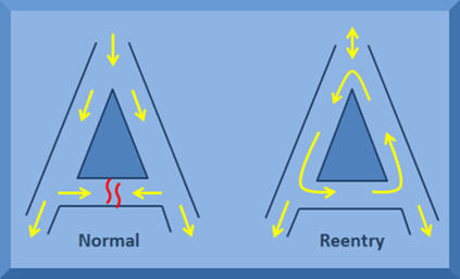
Fig. 11. A classical reentry circuit.

For this example, a classical reentry circuit was built. First, a 12x15 board was constructed and then selected cells were deleted in order to create the specific scheme. Then the primitives were linked together. Next, the cells on the right side of the board were set to a prolonged total repolarization time (RP=250ms) compared to the cells of the left side (RP=110ms), by altering the AP’s phase 2 duration of the cells. The generator cell on the top was adjusted to produce a stimulus every 251ms. In that way, after the first cycle of stimulation, the second wave will meet a "refractory block" of cells on the right branch, while it will continue to travel undisturbed on the left branch. Thus, when the stimulus reaches the right side from the left direction, the lagged right cells will have already been repolarized allowing the wave to enter from the bottom direction (Figure 12(A-I)).

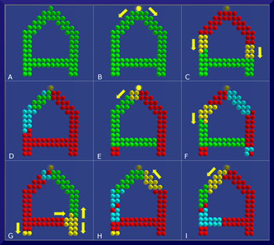
Fig. 12. A) An altered 12x15 board after the deletion of some cells. B) Initiation of simulation. The top cell is a generator cell. C) Propagation from the top to the bottom. D) The cells on the left start being repolarized, while the cells on the right stay in plateau phase. E) The cells on the left and center are resting and the new wave has begun from the top. F) Cells on the right begin to repolarize (light blue) from top to bottom, while the stimulus (yellow) moves downwards on the left. G) Cells on the left branch enter plateau phase. The stimulus reaches the right side and meets cells in rest. H) The yellow wave enters the right side moving from the bottom to the top. There, it meets cells in rest. I) Reentrance; the wave continues to the left side, completing a full circle.

Another example of reentry circuit is shown through Figure 13(A-C). The Kill Cell option was used in order to create two strips of necrotic tissues. The cells placed above and below the black strips have a late repolarization, allowing a stimulus reentrance coming from the cells at center after a cycle. A schematic diagram of the CEAS is shown in Figure 14.

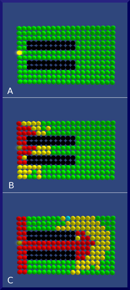
Fig. 13. A). Propagation begins from the left. Black rows represent necrotic areas. B) Wave moves to the right of the board. C) After a cycle, the wave enters the top and bottom pathways, finding cells at rest and strikes back to the left of the board.

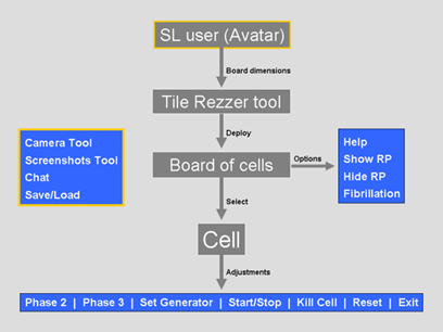
Fig. 14. Overview of CEAS.

4. Discussion

The simulator described here is able to reproduce normal and pathological behavior or the myocardial cells. A cellular DFA model with four states is used to describe the AP phase of each cell. The transmission of the stimulus is governed by a probabilistic model and the transition between the states is time dependent. The impulse propagation across the automata differs from the actual electrical activity of the cardiac tissue. While the reaction-diffusion models are capable on approaching the behavior of the cell’s membrane, they require high computational needs and complex programming techniques, making them impractical for use in mid-level educational simulations. Ionic cardiac models take too much time, even on modern hardware, for a very short simulation (few seconds) of cardiac activity [36]. The other group of diffusion models is based on representing the tissue as a network of cellular automata. This approach is simpler to implement and has a lower computational burden. In combination with a probabilistic model, the membrane’s depolarization depends on both the time spent in rest state and the number of depolarized cells nearby. In this way the propagation is reproduced more naturally, without increasing the calculation time [13].

Whereas CEAS incorporates the flexibility and simplicity of automata concept, its great advantage results from the virtual environment in which lies. Although researchers have recently developed notable cardiac activity simulations using various software tools [15,16,17] none of them can be used inside a VW. Given that the VW are nowadays adopted in pedagogical fields offering many educational benefits through active learning, multimedia and gamification opportunities [37,38], a research effort is desirable to create simulations compatible with virtual environments. CEAS provides a motivation to the user to build its own boards, alter the properties of the AP, and bring to life circuits found in physiology books. The game-like characteristics encourage students to get involved in a constructivist process. With the options provided by the user menu, complex circuits and pathways can be developed. Through experiment and play in the 3D world, we believe that a medical student can visualize and better understand concepts that are difficult to learn by using textbooks without the real-time visual feedback. Furthermore, students can store their cell boards in the SL’s inventory case so they can be easily used again or shared among other users. Users with programming skills can also improve the simulator’s code and share a modified version of CEAS with the virtual community.

5. Conclusions

We presented the programming principles and features of the Cardiac Electrical Activity Simulator, an automata-based educational tool for studying myocardial cell networks in Second Life. CEAS is primarily a student tool providing the flexibility to design and build a tissue of cardiac cells and adjust the parameters of the propagation. The advantages of the on line 3D environment in which the simulator functions, add a great e-learning potential to the CEAS, while making it easier for future improvements by the SL’s user community.

References

1. Palizvan MR, Nejad MR, Jand A & Rafeie M. Cardiovascular physiology misconceptions and the potential of cardiovascular physiology teaching to alleviate these. Med Teach 2013; 35(6): 454-8.
2. Ziv A, Ben-David S & Ziv M. Simulation based medical education: an opportunity to learn from errors. Med Teach 2005; 27(3): 193-9.
3. Morgan PJ, Cleave-Hogg D, Desousa S & Lam-McCulloch J. Applying theory to practice in undergraduate education using high fidelity simulation. Med Teach 2006; 28(1): e10-5.
4. Hodgkin AL & Huxley AF. A quantitative description of membrane currents and its application to conduction and excitation in nerve. J Physiol 1952; 117(4): 500-44.
5. Barkley D. A model for fast computer-simulation of waves in excitable media. Physica D 1991; 49(1-2): 61-70.
6. Di Francesco D & Noble D. A model of cardiac electrical activity incorporating ionic pumps and concentration changes. Philos Trans R Soc Lond B Biol Sci 1985; 307(1133): 353-98.
7. Luo CH & Rudy Y. A dynamic model of the cardiac ventricular action potential. I. Simulations of ionic currents and concentration changes. Circ Res 1994; 74(6): 1071-96.
8. Beeler G & Reuter H. Reconstruction of the action potential of ventricular myocardial fibers. J Physiol 1977; 268(1): 177-210.
9. Chorro Gascó FJ. Mathematical Modeling and Simulations to Study Cardiac Arrhythmias. Rev Esp Cardiol 2005; 58(1): 6-9.
10. Chay TR. Proarrhythmic and antiarrhythmic actions of ion channel blockers on arrhythmias in the heart: model study. Am J Physiol 1996; 271(1 Pt 2): H329-56.
11. Gerhardt M, Schuster H & Tyson JJ. A cellular automation model of excitable media including curvature and dispersion. Science 1990; 247(4950): 1563-6.
12. Plonsey R & Barr RC. (1987). Mathematical modeling of electrical activity of the heart. J Electrocardiol 20(3): 219-26.
13. Bub G & Shrier A. Propagation through heterogeneous substrates in simple excitable media models. Chaos 2002; 12(3): 747-53.
14. Alonso Atienza F, Requena Carrión J & García Alberola A et al. A Probabilistic Model of Cardiac Electrical Activity. Rev Esp Cardiol 2005; 58(1): 41-7.
15. Ye P, Entcheva E, Smolka SA & Grosu R. Modelling excitable cells using cycle-linear hybrid automata. IET Syst Biol 2008; 2(1): 24-32.
16. Bartocci E, Corradini F, Entcheva E, Grosu R & Smolka SA. CellExcite: an efficient simulation environment for excitable cells. BMC Bioinformatics 2008; 9 (Suppl 2): S3.
17. Khan MS, Yousuf S. A cardiac electrical activity model based on a cellular automata system in comparison with neural network model. Pak J Pharm Sci. 2016 Mar; 29(2): 579-84.
18. Balakrishnan M, Chakravarthy VS, Guhathakurta S. Simulation of Cardiac Arrhythmias Using a 2D Heterogeneous Whole Heart Model. Front Physiol. 2015 Dec 21; 6: 374. doi: 10.3389/fphys.2015.00374. eCollection 2015.
19. Bell M. Toward a definition of virtual worlds. JVWR 2008; 1(1): 2-5.
20. Schroeder R. Defining virtual worlds and virtual environments. JVWR 2008; 1(1): 2-5.
21. Second life - Genome Island Sim. Available at: http://slurl.com/secondlife/Genome/149/153/35 [Access date: 01.08.2016]
22. Second Life - Anatomica, American Cancer Society. Available at:http://slurl.com/secondlife/American%20Cancer%20Society/85/192/2009[Access date: 01.08.2016]
23. Second Life - Evergreen Island. Available at: http://maps.secondlife.com/secondlife/Evergreen%20Island%203/36/204/30 [Access date: 01.08.2016]
24. Second Life - OSU Medical Center. Available at:http://slurl.com/secondlife/OSU%20Medicine/214/130/25[Access date: 01.08.2016]
25. Papadopoulos L, Pentzou AE, Louloudiadis K & Tsiatsos TK. Design and evaluation of a virtual patient for pediatric dentistry in virtual worlds. J Med Internet Res 2013; 15(10): e240.
26. Hansen MM, Murray PJ & Erdley WS. The potential of 3-D virtual worlds in professional nursing education. Stud Health Technol Inform 2009; 146: 582-6.
27. Conradi E, Kavia S, Burden D, Rice A, Woodham L, Beaumont C, Savin-Baden M & Poulton T. Virtual patients in a virtual world: Training paramedic students for practice. Med Teach 2009; 31(8): 713-20.
28. Wiecha J, Heyden R, Sternthal E & Merialdi M. Learning in a virtual world: Experience with using second life for medical education. J Med Internet Res 2010; 12(1): e1.
29. Despopoulos AD & Silbernagl S. Color Atlas of Physiology. 5th edition. New York, Thieme; 2003, p. 192-5.
30. Klabunde RE. Cardiovascular physiology concepts. 2nd edition. Lippincott Williams & Wilkins; 2011, p. 16-20.
31. Mohrman DE & Heller LJ. Cardiac abnormalities. In: Mohrman DE, Heller LJ, editors. Cardiovascular Physiology. 7th edition. McGraw-Hill; 2010.
32. Strachey C & Wadsworth CP. Continuations: A Mathematical Semantics for Handling Full Jumps. HOSC 2000; 13(1-2): 135-152.
33. Cardiac Electrical Activity Simulator website. Available at:http://grimore.org/secondlife/cardiac_electrical_activity[Access date: 02.08.2016]
34. CEAS in Second Life’s Marketplace. Available from: https://marketplace.secondlife.com/p/WaS-K-LP-Cardiac-Electrical-Activity-Simulator-CEAS/5167720 [Access date: 02.08.2016]
35. Gaztañaga L, Marchlinski FE & Betensky BP. Mechanisms of Cardiac Arrhythmias. Rev Esp Cardiol 2012; 65(2): 174–185.
36. Mitchell L. Performance Optimisations for CARP: A dCSE project. 2010. Available at: http://www.hector.ac.uk/cse/distributedcse/reports/carp/carp.pdf
37. Ghanbarzadeh R, Ghapanchi AH. Applied Areas of Three Dimensional Virtual Worlds. In: Dong Hwa Choi, Amber Daley-Hebert, Juddi Simmons Estes, editors. Emerging Tools and Applications of Virtual Reality in Education. IGI Global; 2016, p. 26-45.
38. McCoy L, Lewis JH, Dalton D. Gamification and Multimedia for Medical Education: A Landscape Review. J Am Osteopath Assoc 2016 Jan; 116(1): 22-34. doi:10.7556/jaoa.2016.003