The Approximate Calculation of the Roots of Algebraic Equation Through Monte Carlo Method

Vahid Mirzaei Mahmoud Abadi^{1, *}, Shila Banari Bahnamriri²

¹Faculty of Physics, Shahid Bahonar University of Kerman, Kerman, Iran

²Tabari Institute of Higher Education of Babol, Babol, Iran

Abstract

Finding the root of nonlinear algebraic equations is an issue usually found in engineering and sciences. This article presents a new method for the approximate calculation of the roots of a one-variable function through Monte Carlo Method. This method is actually based on the production of a random number in the target range of the root. Finally, some examples with acceptable error are provided to prove the efficiency of this method.

Keywords

Monte Carlo, Root Finding, Nonlinear Algebraic Equation

Received:June 10, 2016
Accepted: August 12, 2016
Published online: August 25, 2016

@ 2016 The Authors. Published by American Institute of Science. This Open Access article is under the CC BY license. http://creativecommons.org/licenses/by/4.0/

1. Introduction

Regarding the recent advances in computer science and the growth of applied software programs for calculating and simulating the complex problems in different sciences, computer methods are used besides the traditional ones as one of the basic methods of science generation.

Many math problems cannot be solved analytically to find an exact answer. In most cases, the only way to describe the behavior of the answer to a problem is to approximate that problem with a numerical method so as to create numbers which can represent the answer to the problem. Numerical methods are used as an alternative to solve more complex problems.

In other words, numerical analysis or calculation studies the methods and algorithms which use numerical approximates (versus analytic answers) for math problems. One of the important and noticeable topics in different sciences that have not been solved completely yet is finding the roots of algebraic equations. Numerical calculations aim to look for some methods of finding approximate roots for each equation. The issue of finding the roots of nonlinear algebraic equations can be often found in sciences and engineering. Numerical root-finding methods use iteration, producing a sequence of numbers that hopefully converge towards a limit, which is a root. The first values of this series are initial guesses. Many methods compute subsequent values by evaluating an auxiliary function on the preceding values. The limit is thus a fixed point of the auxiliary function, which is chosen for having the roots of the original equation as fixed points.

In this regard, some other methods have been introduced to solve algebraic methods in recent years except the common ones like distance …, the Newton method, the tangential chord method and the fixed point method. One of those methods is the Petkovic method (used for finding the recurrent roots of polynomial equations) and the Newton-like iteration method. However, one of the basic and obvious problems in those methods is to find the initial amount which should be adequately close to the real answer. Finding the initial amount is so difficult and tiring, though. Some other new models like the Adomian decomposition method or ADM (Applied Discrete Mathematics) and HPM (Homotopy Perturbation Method) as well as their overgeneralizations have been recently introduced besides the methods mentioned before.

These methods are all almost the same, which makes finding the answer to an equation for larger n’s harder and more complicated. Therefore, this article tries to present an applicable and simple method for the approximate calculation of the roots of algebraic equations through the Monte Carlo calculation method.

2. Materials and Methodology

2.1. Summery of Other Methods

2.1.1. Bisection Method

The simplest root-finding algorithm is the bisection method. It works when f is a continuous function and it requires previous knowledge of two initial guesses, a and b, such that f(a) and f(b) have opposite signs. Although it is reliable, it converges slowly, gaining one bit of accuracy with each iteration.

2.1.2. False Position

The false position method, also called the regula falsi method, is like the secant method. However, instead of retaining the last two points, it makes sure to keep one point on either side of the root. The false position method can be faster than the bisection method and will never diverge like the secant method, but fails to converge under some naive implementations. Ridders' method is a variant on the false-position method that also evaluates the function at the midpoint of the interval, giving faster convergence with similar robustness.

2.1.3. Interpolation

Regula falsi is an interpolation method because it approximates the function with a line between two points. Higher degree polynomials can also be used to approximate the function and its root, while bracketing the root. For example, Muller's method can be easily modified so that rather than always keeping the last 3 points, it tracks the last two points to bracket the root and the best current approximation. Such methods combine good average performance with absolute bounds on the worst-case performance.

2.2. A Review of the Monte Carlo Method

Monte Carlo methods are a class of computational algorithms dependent on recursive random sampling for calculating the related results. These methods are often used for physical simulation, computational physics, computational chemistry, and the numerical integral calculation of mathematical and statistical systems. Since being dependent on repeated calculations and random or pseudo-random numbers, Monte Carl methods are suitable for the calculations done by computer. These methods are considered to be used where calculating an exact answer through the deterministic algorithm proves impossible.

The important point in Monte Carlo methods is the use of random numbers, which is per se a long story in computational physics.

Creating a random number follows a specific mathematical distribution which is tried to be consistent i.e. the intended numbers should be consistently created in the target phase space. However, there are some other distributions which purposefully deal with the creation of random numbers like the exponential distribution, the Gosse distribution etc; consistent distribution is also used in the creation of the Gosse functions, which is due to the fact that sometimes it is needed to create numbers within a limited range in simulation to reduce the simulation time.

One of the basic uses of Monte Carlo methods in numerical calculations is the numerical calculation of the integral. In this method, the integration limit and a general area (range) are specified first. Then, a point in the general area is chosen through creating a random number. If the selected point lies inside the target area (under the integral), it will be acceptable; otherwise, it won’t. If this process is repeated many times, the number of the acceptable points divided by the total number of the repetition times will be a scale of the area under the integral. In this article, the Monte Carlo method was used for the approximate calculation of the roots of algebraic equations.

2.3. The Numerical Solution Algorithm of the Equation Through the Monte Carlo Method

Finding the root of single-variable equations always has three limitations: 1) the root should be looked for in a pre-determined range i.e. the function y=F(x) in the range [a,b], in which a is smaller than b, should be consistent, 2) there should be a root in that range i.e. 0˃ F(a).F(b), 3) the equation root in that range should be unique.

Given that the function F(x) meets those conditions; such problems will be numerically solved through creating random numbers made by the computer program Fortran 90 and the function Ran3.

It should be first supposed that the function F(x) has at least one root. In this case, a program should be written to create a number between a and b and name it c. Then it should compare the sign F(c) with the two sign of the function F(x) at the first and last points of the defined function (points a and b). If F(c) and F(a) have the same sign, the value of c can lies in a and the new range in which the root should be sought will be [c,b]. Otherwise, F(c) and F(b) will have the same sign and b will be replaced by c leading to the creation of the new range [a,c]. This process will continue until the error is acceptable. This convergence towards the root is illustrated in figure (1).

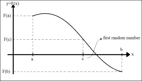
Figure 1. The process of convergence towards the function root through creating random numbers.

The roots of the equation f(x)=x³-2x²-5 were, for instance, calculated for the above algorithm by the written program. This function is defined in the range [2, 3] and is brought in figure (2).

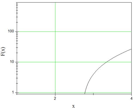
Figure 2. The function curve of F(x)=x³-2x²-5 by Origin (computer program).

Program root find

------------------------------

external f

real a,b,c

idum=7.

i=0

eps=0.0001

a=2.0

b=3.0

10 c=a+(b-a)*ran3(idum)

i=i+1

if(f(a)*f(c).gt.0)then

a=c

else

b=c

endif

if (abs(f(c)).lt.eps)then

write(*,*)'############'

write(*,*)'Final Root Is=',c

write(*,*)'F(x) Is=',f(c)

write(*,*)'############'

else

write(*,*)' ','value of x',' ','F(x)',' *','Num of step'

print*,c,f(c),i

goto 10

endif

End

function f(x)

f=x**3-2*x**2-5

return

end

One can determine precision of the root which has been found in the range [a,b] by the length of this range. Parameter eps in the above program is the precision of the answer. The output of the program is 2.6906 with an error of less than 0.0001, which is confirmed through drawing the curve by Origin and finding the cross-point with the axis x.

The next example is the calculation of the root of the equation F(x)=x-0.5cos(x) which is defined in the range [1,0] and has an analytical answer. This curve is brought in figure (3).

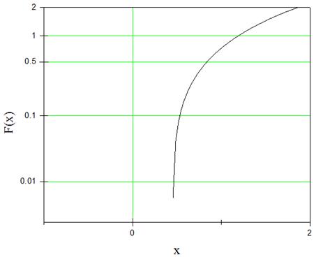
Figure 3. The function curve of F(x)=x-0.5cos(x) by Origin.

3. Result and Discussion

According Monte Carlo method for root finding the speed of converge to the root in this method chancy in compare to another methods. Because the range which root is located in is related to the random number. If the random numbers be near the root chancy this algorithm will converge rapidly and vise versa. The error of this method is determined by the size of range [a,b].

4. Conclusion

In this article, the Monte Carlo method was used to find the root of nonlinear equations through creating random numbers for the first turn. This method is so simple and useful in comparison to other methods that the approximate answer to nonlinear equations can be obtained with a high degree of precision through this method. The other advantages of this method are its not being repeated, not needing a starting point, and providing an answer with an acceptable error. The speed of converge to answer in this method is depended to the range [a,b] and algorithm of produce random number. This method lead to correct root like another methods and so this method can used as new method for root finding.

References

1. L. Petkovic et al., On the conctruction of simultaneous method for multiple zeros, Non-Linear Anal., Theory, Meth. Appl. 30(1997) 669-676.
2. J.H. He, Newton-like iteration method for solving algebraic equations, Commun. Nonl-Iinear Sci. Numer. Simulation 3(2) (1998).
3. J.H. He, Improvement of Newton-like iteration method, Int. J. Nonlinear Sci. Numer. Simulation 1(2) (2000) 239-240.
4. T. Yamamoto, Historical development in convergence analysis for Newtons and Newt on-loke method, J Comput, Appl, Math,. 124 (2000) 1-23.
5. Adomian G, Rach R., On the solution of algebraic equations by the decomposition method, Math. Anal. Appl., 105, (1985), 141-166.
6. S. Abbasbandy, M.T. Darvishi, A numerical solution of Burgers equation by modified Adomian method, Appl. Math. Comput., 163 (2005), 1265-1272.
7. K. Abbaoui, Y. Cherruault, Convergence of Adomian’s Method Applied to Nonlinear Equations, Math. Comput. Model., 20(9), (1994), 69-73.
8. E. Babolian, J. Biazar, Solution of nonlinear equations by modified Adomian decomposition method, Appl. Math. Computation, 132 (2002) 167-172.
9. E. Babolian, J. Biazar, On the order of convergence of Adomian method, Applied Mat- hematics and Computation, 130, (2002), 383-387.
10. E.Babolian, A. Davari, Numerical implementation of Adomian decomposition method, Appl. Math. Comput., 153, (2004), 301-305.
11. Y. Cherruault, Convergence of Adomian’s Method, Kybernetes, 8(2), 1998, 423-426.
12. Cherruault Y, Adomian G., Decomposition methods: a new proof of convergence.Math. Comput. Modell., 18, (1993), 103-106.
13. J.H. He, Homotpy perturbation method, Comp. Math. Appl. Mech. Eng. 178 (1999) 257–262.
14. J.-H. He, A coupling method of homotopy technique and perturbation technique for Nonlinear problems, Intm J Nonlinear Mech. 35(1) (2000) 37-43.
15. S. Abbasbandy, Modified homotopy perturbation method for nonlinear equation and Comparison with Adomian decomposition method, Applied Mathemetics and comput172 (2006) 431-438.
16. Richard Belman, Perturbation Techniques in Mathematics, Physics, and Engineering. Dover Pub. Inc., New York,1972.
17. Brown. J. W, Churchill. R. V, Coplex Variables and Applications, Sixth Editoin, McGraw-Hill, 1996.
18. T. Yamamoto, Historical development in convergence analysis for Newton’s and Newton-likemethods, J. Comput. Appl. Math. 124 (2000) 1–23.
19. Ji. Huan He, Anew iteration method for solving algebraic equations, Appl. Math. 135 (2003) 81-84.
20. S. Abbasbandy, Improving Newton-Raphson method for nonlinear equations by mod- Ified Adomian decomposition method, Appl. Math. 145 (2003) 887-893.
21. Changbum chun, Anew iterative method for solving nonlinear equations, Appl. Math, 178 (2006) 415-422.
22. S. Abbsbandy,Y. Tan, S.J Liao, Newton-Homotopy analysis method for nonlinear eq-Uations,Applied Mathemetics and comput. 188 (2007) 1794=1800.
23. E. Babolian, T. Lotfi, F. M. Yaghoobi, Solving no linear equation by perturbation technique and Lagrange expansion, extended abstract of the 18th seminar on mathematical analysis and it application, 2009, pp 154-157.
24. Krandick, W., Mehlhorn, K. "New Bounds for the Descartes Method"; Journal of Symbolic Computation, 41, (2006), 49-66.
25. Sharma, V. "Complexity Analysis of Algorithms in Algebraic Computation"; Ph.D. Thesis, Department of Computer Sciences, Courant Institute of Mathematical Sciences, New York University, 2007.
26. Cordero A, Torregrosa JR (2006) Variants of Newton’s method for functions of several variables. Appl Math Comput 183:199–208.
27. Cordero A, Hueso JL, Martínez E, Torregrosa JR (2012) Increasing the convergence order of an iterative method for nonlinear systems. Appl Math Lett 25:2369–2374.
28. Grau-Sánchez M, Noguera M (2012) A technique to choose the most efficient method between secant method and some variants. Appl Math Comput 218:6415–6426.
29. Petkovi ́ MS, Neta B, Petkovi ́ LD, Džuni ́ J (2013) Multipoint methods for solving nonlinear equations. Elsevier, Boston.
30. Sharma JR, Arora H (2014) Efficient Jarratt-like methods for solving systems of nonlinear equations. Calcolo 51:193–210. doi: 10.1007/s10092-013-0097-1.
31. Sharma JR, Guha RK, Sharma R (2013) An efficient fourth order weighted-Newton method for systems of nonlinear equations. Numer Algorithms 62:307–323.