
International Journal of Mathematics and Computational Science, Vol. 1, No. 5, October 2015 Publish Date: Aug. 7, 2015 Pages: 317-323
Comparison of Mesh-Based and Meshless Methods for Solving the Mathematical Model Arising of Launching Devices During the Firing
S. Sarabadan*, M. Kafili
Departeman of Mathematics, Imam Hossein University, Tehran, Iran
Abstract
In this paper, we apply different mesh-based and meshless methods for solving matrix system carried out from modelling the rockets stability during the firing. Sloped rocket launch and its stability during the firing is one of the most important kinds of defense instruments. The rockets stability during the firing path especially when they are unguided is very important for firing precision. Two mesh-based schemes as finite difference and B-spline methods and two meshless schemes as radial basis function (RBF) and radial basis functions based on finite difference (RBF-FD) are employed for solving underlying system. Numerical results are presented as tabular forms. They show that computational errors and CPU time for RBF-FD as a meshless method are better than other methods.
Keywords
Mesh-Based Method, Meshless Method, Sloped Rocket Launch
Received: July 5, 2015
Accepted: July 22, 2015
Published online: August 8, 2015
@ 2015 The Authors. Published by American Institute of Science. This Open Access article is under the CC BY-NC license. http://creativecommons.org/licenses/by-nc/4.0/
1. Introduction
Numerical methods can be divided into two major categories: Mesh-based and Meshless methods. The traditional mesh-based methods such as finite difference method (FDM) and B-spline method are widely used in many fields of science and engineering and some powerful packages have been developed for them. Some limitations in mesh generation, remeshing and constructing the approximation scheme tend the public interests to apply the meshless methods that remove the limitations of classical mesh-based methods. Meshless methods have been proved to treat scientific and engineering problems efficiently. They apply only a cloud of points without any information about nodal connections. One of the most popular meshless methods is constructed by radial kernels as basis called radial basis function (RBF) method. It is (conditionally) positive definite, rotationally and transnationally invariant. In other hand, system matrices with high condition numbers often result in this method is one of the most defense of it. These properties make its application straightforward specially for approximation problems with high dimensions. RBFs include two useful characteristics: a set of scattered centers with possibility of selecting their locations and existence of a free positive parameter known as the shape parameter. "Shape parameter" is a customary name for RBF free parameter in the literature, but it is also called scale parameter, width, or (reciprocal of the) standard deviation. A progress version of RBF method is radial basis function based on finite difference that is the local version of RBF method. This method is very useful for solving systems with initial perturbed or random conditions [1,2].
Here, we intend to compare both mesh-based and meshless methods for solving a system of first order differential equations arising of launching devices oscillations during the firing. Due to, the finite difference and B-spline methods as mesh-based schemes and RBF and RBF-FD methods as meshless schemes are compared in accuracy and CPU time. The rest of the paper is organized as follows: The system of first order differential equations arising of launching devices oscillations during the firingis explained in Section 2. In the Section 3, a brief review on the four mentioned methods is presented, then applied for underlying system. The numerical results are shown in the Section 4 and methods are compared and interpreted in tabular form.
2. The Mathematical Model
The study of launching device oscillations during the firing is necessary for the design of precise and efficient rocket-launching device systems, especially in the case of unguided rockets. We suppose that the launching device and the moving rocket form a complex oscillating system that join together a sum of rigid bodies bound by elastic elements (the vehicle chassis, the tilting platform and the rockets in the containers) [3]. Some authors have been considered all forces and moments to a real analysis of problem [3,4]. It results in a matrix form of the second order differential equations system that describes the matrix form of dynamic equations of the rocket-launching device system motion.
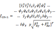
Suppose the independent unknown dynamic variables of the rocket-launching device system motion can be presented in the form of the following column vector [4]:
![]() (2.1)
(2.1)
where the vehicle chassis translation ![]() , the vehicle chassis rotation
, the vehicle chassis rotation ![]() (the chassis pitch movement), the vehicle chassis rotation
(the chassis pitch movement), the vehicle chassis rotation ![]() (the chassis rolling movement), the tilting platform rotation
(the chassis rolling movement), the tilting platform rotation ![]() (the gyration movement around the vertical axes), the tilting platform rotation
(the gyration movement around the vertical axes), the tilting platform rotation ![]() (the pitch movement) and the rocket translation
(the pitch movement) and the rocket translation ![]() , are components of
, are components of ![]() . So, one can obtain the matrix form of the second order differential equations system that describes the rocket-launching system components motion:
. So, one can obtain the matrix form of the second order differential equations system that describes the rocket-launching system components motion:
![]() (2.2)
(2.2)
Where ![]() is the matrix of the velocities coefficients,
is the matrix of the velocities coefficients, ![]() ;
; ![]() is the matrix of the unknown variables coefficients
is the matrix of the unknown variables coefficients ![]() .
. ![]() is the matrix of the coefficients for the nonlinear combinations of the unknown variables:
is the matrix of the coefficients for the nonlinear combinations of the unknown variables:
 (2.3)
(2.3)
For more information about the components of matrices (1.3), that can be specified randomly, one can see [3,4]. And, the ![]() is the matrix of the external forces that acts on the system:
is the matrix of the external forces that acts on the system:
![]() (2.4)
(2.4)
The vector (2.4) is used to express the influence of the external forces on the motion system. In this vector, the first term corresponds to the weight force, the second term corresponds to the rocket thrust and the last term to the rocket jet force [4].
The mathematical model can be used to study any launching device like the underlying problem [3,4]. For solving the underlying system, at the first, one can be reduce the system of second order differential equations (2.2) to a system of first order differential equations [4], we must introduce the following variables:
![]() (2.5)
(2.5)
![]() (2.6)
(2.6)
![]() (2.7)
(2.7)
![]() (2.8)
(2.8)
![]() (2.9)
(2.9)
![]() (2.10)
(2.10)
Using those new variables (2.5)-(2.10), the unknown variables vector can be presented as following [4]:
![]() (2.11)
(2.11)
Using the notations (2.5)-(2.10) and the vector (2.11), as well as the equation (2.2), we obtain the new matrix form of the first order differential equations, which describes the motion of the rocket-launching device system:
![]() (2.12)
(2.12)
where,
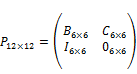
![]() (2.13)
(2.13)
![]()
Which ![]() ,
, ![]() and
and ![]() are zeros matrices and as mentioned before other blocks are the random matrices that their elements are random values that impose the launching device during the firing. Here, we solve the matrix system (2.12) by applying radial basis functions. The 6 scalar equations are necessary to calculate the
are zeros matrices and as mentioned before other blocks are the random matrices that their elements are random values that impose the launching device during the firing. Here, we solve the matrix system (2.12) by applying radial basis functions. The 6 scalar equations are necessary to calculate the ![]() unknown variables that describe the movement of the rocket-launching device system during firing (
unknown variables that describe the movement of the rocket-launching device system during firing (![]() ) while the other scalar equations allow to compute the evolutions of the differentials of
) while the other scalar equations allow to compute the evolutions of the differentials of ![]() main unknown variables defined with (2.5)-(2.10) [4].
main unknown variables defined with (2.5)-(2.10) [4].
3. A Brief Review on Mesh-Based and Meshless Methods
In this section we proposed a summary of the applied mesh-based schemes: FDM and B-spline schemes, and meshless methods: RBF and RBF-FD schemes. So, these methods apply to solve the system matrix (2.12).
3.1. Mesh-Based Methods: FDM
Our goal is to approximate solutions to differential equations, i.e., to find a function (or some discrete approximation to this function) which satisfies a given relationship between various of its derivatives on some given region of space and/or time, long with some boundary conditions along the edges of this domain. In general this is a difficult problem and only rarely can an analytic formula be found for the solution. A finite difference method proceeds by replacing the derivatives in the differential equations by finite difference approximations. This gives a large algebraic system of equations to be solved in place of the differential equation, something that is easily solved on a computer[5].
Let ![]() represent a function of one variable that, unless otherwise stated, will always be assumedto be smooth, meaning that we can differentiate the function several times and each derivative is a well-defined bounded function over an interval containing a particular point of interest
represent a function of one variable that, unless otherwise stated, will always be assumedto be smooth, meaning that we can differentiate the function several times and each derivative is a well-defined bounded function over an interval containing a particular point of interest ![]() .
.
Suppose we want to approximate ![]() by a finite difference approximation based only on values ofu at a finite number of points near
by a finite difference approximation based only on values ofu at a finite number of points near ![]() . One obvious choice would be to use
. One obvious choice would be to use
![]() (3.1.1)
(3.1.1)
for some small value of ![]() . This is motivated by the standard definition of the derivative as the limitingvalue of this expression as
. This is motivated by the standard definition of the derivative as the limitingvalue of this expression as![]() . Note that
. Note that ![]() is the slope of the line interpolating
is the slope of the line interpolating ![]() at thepoints
at thepoints ![]() and
and ![]() .
.
The expression (3.1.1) is a one-sided approximation to ![]() since
since ![]() is evaluated only at values of
is evaluated only at values of![]() .Another one-sided approximation would be
.Another one-sided approximation would be
![]() (3.1.2)
(3.1.2)
Each of these formulas gives a first order accurate approximation to ![]() , meaning that the size of the error is roughly proportional to
, meaning that the size of the error is roughly proportional to ![]() itself.
itself.
Another possibility is to use the centered approximation
![]() (3.1.3)
(3.1.3)
This is the slope of the line interpolating ![]() at
at ![]() and
and ![]() , and is simply the average of the two one-sided approximations defined above. It should be clear that we would expect
, and is simply the average of the two one-sided approximations defined above. It should be clear that we would expect![]() to give a better approximation than either of the one-sided approximations. In fact this gives asecond order accurate approximation, the error is proportional to
to give a better approximation than either of the one-sided approximations. In fact this gives asecond order accurate approximation, the error is proportional to ![]() and hence is much smaller than the error in a first order approximation when
and hence is much smaller than the error in a first order approximation when ![]() is small.Simplicity of applying it is one of the important advantage and the mesh generation and remeshing spatially for complex domains is one of its important disadvantages.
is small.Simplicity of applying it is one of the important advantage and the mesh generation and remeshing spatially for complex domains is one of its important disadvantages.
For solving the matrix system (2.12) by the FDM, at the first, we discretize the interval ![]() for
for ![]() with
with![]() nodes with the step size
nodes with the step size ![]() so, by collocating (2.12) and approximating the components of
so, by collocating (2.12) and approximating the components of ![]() with the (3.1.3), so that for the nodal points
with the (3.1.3), so that for the nodal points ![]() :
:
![]() (3.1.4)
(3.1.4)
Where at the first node ![]() and the end node
and the end node ![]() the values of
the values of ![]() is determined randomly and zero respectively. This scheme leads to
is determined randomly and zero respectively. This scheme leads to![]() multi-diagonal matrix system. By solving the resulting systems one can obtain the solution in nodal points.
multi-diagonal matrix system. By solving the resulting systems one can obtain the solution in nodal points.
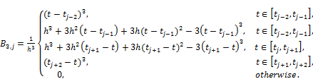
3.2. Mesh-Based Methods: B-Spline Method
In this section we describe the B-spline collocation method to use the matrix system (2.12). Le t![]() be the partition in
be the partition in ![]() . We define the cubic B-spline for
. We define the cubic B-spline for ![]() by the following relation,
by the following relation,
 (3.2.1)
Our numerical treatment for solving (2.12) using the collocation method with cubic B-splines is to find an approximate solution ![]() to exact solution
to exact solution ![]() in the form,
in the form,
![]() (3.2.2)
(3.2.2)
Where ![]() are unknown time dependent parameters to be determined from the boundary conditions and collocationof the differential equation. The values of
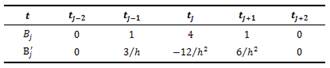
are unknown time dependent parameters to be determined from the boundary conditions and collocationof the differential equation. The values of ![]() and its two derivatives may be tabulated as in Table1.
and its two derivatives may be tabulated as in Table1.
Table 1. Values of ![]() and its first derivative at the nodal points.
and its first derivative at the nodal points.
Using approximate function (3.2.2) and cubic B-spline (3.2.1), the approximate values at the knots of ![]() and itsderivatives are determined in terms of the time dependent parameters
and itsderivatives are determined in terms of the time dependent parameters ![]() as,
as,
![]() (3.2.3)
(3.2.3)
![]() (3.2.4)
(3.2.4)
Now for solving the matrix system (2.12) suppose that for each components of ![]() the
the ![]() satisfies the (2.12) plus the boundary conditions for
satisfies the (2.12) plus the boundary conditions for ![]() (that its value determined randomly) and
(that its value determined randomly) and ![]() (that its value can specified zero because of it is the end of process). This scheme leads us to the
(that its value can specified zero because of it is the end of process). This scheme leads us to the ![]() tri-diagonal matrix system which by solving them one can obtain the solution of (2.12).
tri-diagonal matrix system which by solving them one can obtain the solution of (2.12).
3.3. Meshless Methods: RBF
One of the most popular meshless methods is constructed by radial kernels as basis called radial basis function (![]() ) method. It is (conditionally) positive definite, rotationally and translationally invariant. These properties make its application straightforward specially for approximation problems with high dimensions. Some of the well-known RBFs are as follows,
) method. It is (conditionally) positive definite, rotationally and translationally invariant. These properties make its application straightforward specially for approximation problems with high dimensions. Some of the well-known RBFs are as follows,
![]() (
(![]() ) :
) :![]()
![]() (
(![]() ):
): ![]()
![]() (
(![]() ):
):![]()
where![]() is the Euclidean distance between any two points
is the Euclidean distance between any two points ![]() ,
, ![]() , [1,2]. The
, [1,2]. The ![]() include two useful characteristics: a set of scattered centers
include two useful characteristics: a set of scattered centers ![]() with possibility of selecting their locations and existence of a free positive parameter,
with possibility of selecting their locations and existence of a free positive parameter, ![]() , known as the shape parameter.
, known as the shape parameter.
Assume the ![]() be the shape parameter corresponding to
be the shape parameter corresponding to ![]() center
center ![]() , we use following notation for translation of
, we use following notation for translation of ![]() at
at ![]() center,
center,
![]()
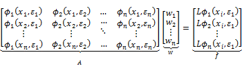
Let data values ![]() are given, the function
are given, the function ![]() will be approximated using a linear combination of translates of a single
will be approximated using a linear combination of translates of a single ![]() so that,
so that,
![]() (3.3.1)
(3.3.1)
where the unknown coefficients ![]() will be determined by collocating (3.3.1) at the same set of centers,
will be determined by collocating (3.3.1) at the same set of centers, ![]() .
.
The shape parameter plays an important role in ![]() , the choice of it controls the shape of the basis functions and interchanges the error and stability of interpolation process. This behavior is manifested as a classical tradeoff between accuracy and stability or Uncertainty Principle [6] which refers to the fact that an RBF approximant can not be accurate and well-conditioned at the same time.
, the choice of it controls the shape of the basis functions and interchanges the error and stability of interpolation process. This behavior is manifested as a classical tradeoff between accuracy and stability or Uncertainty Principle [6] which refers to the fact that an RBF approximant can not be accurate and well-conditioned at the same time.
Two scenarios are available for choosing shape parameters: constant shape parameter (![]() ) strategies that all of shape parameters take the same value and variable shape parameter (
) strategies that all of shape parameters take the same value and variable shape parameter (![]() ) strategies that assign different values to shape parameters corresponding to each center. Many scientists and mathematicians use
) strategies that assign different values to shape parameters corresponding to each center. Many scientists and mathematicians use ![]() in
in ![]() approximations [7,8,9] because of their simple analysis as well as solid theoretical background rather than
approximations [7,8,9] because of their simple analysis as well as solid theoretical background rather than ![]() , but there are numerous results from a large collection of applications [10,11,12,13] indicating the advantages of using
, but there are numerous results from a large collection of applications [10,11,12,13] indicating the advantages of using ![]() .
.
For solving the matrix system (2.12), we approximate the components of ![]() with the
with the ![]() interpolant (3.3.1) so that:
interpolant (3.3.1) so that:
![]() (3.3.2)
(3.3.2)
Where ![]() is constant. By differentiating from (3.10) the components of
is constant. By differentiating from (3.10) the components of ![]() obtained as follows:
obtained as follows:
![]() (3.3.3)
(3.3.3)
Substituting the equations (3.3.2), (3.3.3) in (2.12) and collocating it in same ![]() centers, we obtain
centers, we obtain ![]() system of equations with unknown parameters
system of equations with unknown parameters ![]() . Therefore, one can be approximate the unknown variables
. Therefore, one can be approximate the unknown variables ![]() from equations (3.3.2).
from equations (3.3.2).
3.4. Meshless Methods: RBF-FD
As mentioned before to calculate the derivatives of function ![]() at node
at node ![]() , first we approximate the function
, first we approximate the function ![]() by linear combination of RBFs as (3.3.1), then apply the derivative operator
by linear combination of RBFs as (3.3.1), then apply the derivative operator ![]() on the above RBF interpolant and evaluate it at the desired node location:
on the above RBF interpolant and evaluate it at the desired node location:
![]() (3.4.1)
(3.4.1)
The above formula is a global derivation. That is, to calculate the discretized derivative operator at one node, all the nodes in the domain are used. In RBF-FD method for each stencil, only ![]() nodes out of the
nodes out of the ![]() nodes in the domainare used and the differential operator
nodes in the domainare used and the differential operator ![]() is approximated at the node
is approximated at the node ![]() by a linearcombination of the function values
by a linearcombination of the function values ![]() at the neighboring
at the neighboring ![]() nodes locations:
nodes locations:
![]() (3.4.2)
(3.4.2)
Unlike the conventional FD method, which uses the polynomials of degree ![]() or lessfor computing the weights
or lessfor computing the weights ![]() in above linear combination, RBF-FD method calculatesthese weights by imposing the requirement that the above linear combination must be exact for RBFs,
in above linear combination, RBF-FD method calculatesthese weights by imposing the requirement that the above linear combination must be exact for RBFs, ![]() , centered at each of the node locations
, centered at each of the node locations ![]() . Combining these constraints, the solution for the RBF-FD weights can be determined from the following linear system:
. Combining these constraints, the solution for the RBF-FD weights can be determined from the following linear system:
 (3.4.3)
In our work, the operator ![]() is the first order derivative operator and among radial basis functions, we use Multiquadric (MQ) function. It can be shown that the system matrix
is the first order derivative operator and among radial basis functions, we use Multiquadric (MQ) function. It can be shown that the system matrix ![]() in (3.4.3) for this function is invertible. Now, we use the Maple software and explicitly present the weight coefficients for approximating the first order derivative. In general, assume that set
in (3.4.3) for this function is invertible. Now, we use the Maple software and explicitly present the weight coefficients for approximating the first order derivative. In general, assume that set ![]() be anon-uniform partition of the interval
be anon-uniform partition of the interval ![]() . To approximate first order derivative of function
. To approximate first order derivative of function ![]() at points of
at points of ![]() we apply a three point central scheme:
we apply a three point central scheme: ![]() and [
and [![]() ]. After solving linear system (3.4.3) and suppose that
]. After solving linear system (3.4.3) and suppose that ![]() and c ≫ h the weight coefficients of RBF-FD method for approximating the first derivative of function
and c ≫ h the weight coefficients of RBF-FD method for approximating the first derivative of function ![]() are given as:
are given as:
![]() (3.4.4)
(3.4.4)
Which coincides with the standard central difference approximation to the first derivative with a correction term of order![]() [14].
[14].
Now, we present a scheme for solving the matrix system (2.12). At the first, we approximate the values of components of ![]() in node
in node ![]() by RBF-FD using
by RBF-FD using ![]() and [
and [![]() ], as well as the components of
], as well as the components of ![]() approximate so that:
approximate so that:
![]()
After substituting the weights (3.4.4), one can obtain ![]() tri-diagonal matrix systems results in the solutions in nodal points
tri-diagonal matrix systems results in the solutions in nodal points ![]() .
.
4. Numerical Results
In this Section, we compare both mesh-based and meshless methods based on four mentioned schemes. Our numerical results let us carry out some results about advantages and disadvantages of different methods and finally about mesh-based and meshless methods. All numerical results carried out using Maple software. In all schemes, the matrices ![]() are produced with Maple’s Random function that randomly assigns elements in interval
are produced with Maple’s Random function that randomly assigns elements in interval ![]() for the underlying matrices. The
for the underlying matrices. The ![]() function with the constant shape parameter
function with the constant shape parameter ![]() for
for ![]() is applied for basis function in both RBF and RBF-FD schemes. Support interval is specified as
is applied for basis function in both RBF and RBF-FD schemes. Support interval is specified as ![]() , also the number of nodal points (in meshless schemes: number of centers) are selected so that
, also the number of nodal points (in meshless schemes: number of centers) are selected so that![]() . Based on theoretical and numerical experiments [8,9,10,11] it is clear that increasing
. Based on theoretical and numerical experiments [8,9,10,11] it is clear that increasing ![]() results in more accurate results. The approximation of the components of
results in more accurate results. The approximation of the components of ![]() are shown in tabular forms in tables 2-4 for some
are shown in tabular forms in tables 2-4 for some ![]() , then some interpretations and experiments of applying different approaches are presented. Notice that by passing time (increasing
, then some interpretations and experiments of applying different approaches are presented. Notice that by passing time (increasing ![]() ), the values of oscillations parameters tend to zero. It is clear that output results be different compared with those are presented for other random matrices (2.13), but according to our observations, they are similar to presented results for any random matrices.
), the values of oscillations parameters tend to zero. It is clear that output results be different compared with those are presented for other random matrices (2.13), but according to our observations, they are similar to presented results for any random matrices.
Table 2. Comparison of different schemes for ![]()
| FDM | B-spline method | RBF | RBF-FD | |
|
| -2.0001 | -1.6544 | -0.9563 | -0.7650 |
|
| 0.3999 | 0.2225 | 0.1567 | 0.1198 |
|
| -0.0190 | -0.0122 | -0.0065 | -0.0054 |
|
| -0.1666 | -0.1589 | -0.1011 | -0.0776 |
|
| 0.0795 | 0.0650 | 0.0655 | 0.0400 |
|
| -0.0561 | -0.0444 | -0.0340 | -0.0201 |
|
| -0.0231 | -0.0226 | -0.0121 | -0.0098 |
|
| -0.0990 | -0.0760 | -0.0602 | -0.0341 |
|
| 0.0808 | 0.0685 | 0.0700 | 0.0614 |
|
| 0.0861 | 0.0790 | 0.0502 | 0.0440 |
|
| 0.0902 | 0.0599 | 0.0407 | 0.0384 |
|
| 0.0357 | 0.0309 | 0.0255 | 0.0189 |
| CPU time(second) | 0.37 | 0.21 | 0.45 | 0.09 |
Table 3. Comparison of different schemes for ![]()
| FDM | B-spline method | RBF | RBF-FD | |
|
| -1.0191 | -0.8789 | -0.5950 | -0.4711 |
|
| 0.1391 | 0.1045 | 0.0865 | 0.0705 |
|
| 0.0142 | 0.0103 | -0.0094 | 0.0074 |
|
| -0.3093 | -0.2999 | -0.2374 | -0.2090 |
|
| 0.1577 | 0.1209 | 0.0997 | 0.0413 |
|
| -0.0342 | -0.0268 | -0.0104 | -0.0099 |
|
| 0.0091 | 0.0079 | 0.0043 | 0.0038 |
|
| -0.0788 | -0.0595 | -0.0375 | -0.0214 |
|
| 0.1672 | 0.1544 | 0.1286 | 0.1174 |
|
| 0.0502 | 0.0491 | 0.0205 | 0.0188 |
|
| 0.1399 | 0.1390 | 0.1208 | 0.1186 |
|
| 0.1184 | 0.1096 | 0.0954 | 0.0609 |
| CPU time(second) | 0.37 | 0.21 | 0.45 | 0.09 |
Table 4. Comparison of different schemes for ![]()
| FDM | B-spline method | RBF | RBF-FD | |
|
| -0.0177 | -0.0185 | -0.0054 | -0.0001 |
|
| 0.0391 | 0.0287 | 0.0098 | 0.0019 |
|
| 0.0051 | 0.0048 | 0.0031 | 0.0008 |
|
| -0.1291 | -0.1019 | -0.0848 | -0.0666 |
|
| 0.0886 | 0.0696 | 0.0475 | 0.0109 |
|
| -0.0099 | -0.0087 | -0.0054 | -0.0039 |
|
| -0.0009 | -0.0006 | -0.0005 | -0.0001 |
|
| -0.0502 | -0.0299 | -0.0154 | -0.0076 |
|
| 0.0444 | 0.0390 | 0.0401 | 0.0389 |
|
| 0.1021 | 0.0991 | 0.0868 | 0.0753 |
|
| 0.0608 | 0.0582 | 0.0397 | 0.0115 |
|
| 0.0299 | 0.0289 | 0.0221 | 0.0190 |
| CPU time(second) | 0.37 | 0.21 | 0.45 | 0.09 |
As it is shown in numerical results, the RBF-FD scheme as a meshless method results in less values as solutions because of less computational errors rather than other results. As well as the CPU time in this case is less than others. The RBF scheme as another meshleass method has run ![]() second that is more than CPU time for other methods that its reason is the system matrices with high condition numbers in this scheme. It results in that the mesh-based methods are better than the RBF method as meshless method but the RBF-FD as a meshless method that is produced by combining of FDM and RBF methods has better performance rather than other approaches.
second that is more than CPU time for other methods that its reason is the system matrices with high condition numbers in this scheme. It results in that the mesh-based methods are better than the RBF method as meshless method but the RBF-FD as a meshless method that is produced by combining of FDM and RBF methods has better performance rather than other approaches.
Notations and Symbols
![]() independent unknown dynamic variables of the rocket-launching device system motion
independent unknown dynamic variables of the rocket-launching device system motion
![]() vehicle chassis translation
vehicle chassis translation
![]() chassis pitch movement
chassis pitch movement
![]() chassis rolling movement
chassis rolling movement
![]() gyration movement around the vertical axes
gyration movement around the vertical axes
![]() pitch movement
pitch movement
![]() rocket translation
rocket translation
![]() matrix of the coefficients for the nonlinear combinations of the unknown variables
matrix of the coefficients for the nonlinear combinations of the unknown variables
![]() external forces that acts on the system
external forces that acts on the system
![]() shape parameter
shape parameter
![]() Euclidean distance
Euclidean distance
![]() set of centers
set of centers
![]() derivative of s
derivative of s
![]() derivative of
derivative of ![]()
![]() derivative of
derivative of ![]()
![]() derivative of
derivative of ![]()
![]() derivative of
derivative of ![]()
References
- H. Wendland, Scattered Data Approximation, Cambridge University Press, (2005).
- M. D. Buhmann,Radial Basis Functions: Theory and Implementation, University of Gissen, Cambridge University Press, (2004).
- P. Somoiag, C. Moldoveanu, Numerical research on the stability of launching devices during firing, Defence Technology 9, (2013), 242-248.
- P. Somoiag, F. Moraru, D. Safta, C. Moldoveanu, A mathematical model for the motion of a rocket-launching device system on a heavy vehicle, Military technical academy, Romania, (2012).
- R. J. Leveque, Finite difference methods for differential equations, University of Washington, (2005).
- R. Schaback, Improved error bounds for scattered data interpolation by radial basis functions, Math Comput, 68, (1999), 201-206.
- R. L. Hardy, Multiquadric equations of topography and other irregular surfaces, J Geophys Res, 76, (1971), 1905-1915.
- R. Franke, Scattered data interpolation: tests of some methods, Math Comput, 38, (1982), 181-200.
- C. S. Huang, C. F. Lee, A. D. Cheng, Error estimate, optimal shape factor, and high precision computation of multiquadric collocation method, Eng Anal Bound Elem, 31, (2007), 614-623.
- R. E. Carlson, T. A. Foley, The parameter in multiquadric interpolation, Comput Math Appl, 21, (1991), 29-42.
- E. J. Kansa, R. E. Carlson, Improved accuracy of multiquadric interpolation using variable shape parameters, Comput Math Appl, 24, (1992), 99-120.
- E. J. Kansa, R. C. Aldredge, L. Ling. Numerical simulation of two-dimensional combustion using mesh-free methods, Eng Anal Bound Elem, 33, (2009), 940-950.
- S. A. Sarra, D. Sturgill, A random variable shape parameter strategy for radial basis function approximation methods, Eng Anal Bound Elem, 33, (2009), 1239-1245.
- V. Bayona, M. Moscoso, M. Carretero, M. Kindelan, RBF-FD formulas and convergence properties, Journal of computational physics, 229, (2010), 8281-8295.


