
International Journal of Mathematics and Computational Science, Vol. 1, No. 5, October 2015 Publish Date: Aug. 13, 2015 Pages: 332-338
"Restricted Euler Equations" Model Is Not Very Suitable for Revealing Properties Inherent to Euler Equations
Vladimir A. Dobrynskii*
Institute for Metal Physics of N.A.S.U., Kiev, Ukraine
Abstract
For the restricted Euler equations, we prove the following: 1) If there is a time instant such that the perfect vector alignment between the vorticity vector and the strain matrix eigenvector happens at some point inside the 3D incompressible restricted Euler flow, it continues then permanently and keeps forever in the sense that one happens successively at all points which belong to the given point trajectory generated by the flow. 2) If the aforementioned trajectory exists, then, depending on initial data, one can either blow up for a finite time or not. What is interesting in doing so is that the aforesaid finite-time blow ups can be various and very different. In particular, we found the blow up such that the strain matrix eigenvalues all go at infinity (which can be both positive and negative) whereas the vorticity remains bounded at the same time. Such kind the vorticity behavior should be considered, generally speaking, as slightly unexpected if to take into account the well-known Beale-Kato-Majda (abbr. BKM) criterion for solutions of the genuine Euler equations to blow up at a finite-time. On the other hand, there are solutions to the restricted Euler equations which blow up at a finite time by a scenario similar to that is described in the BKM criterion. Summarizing all what is the aforesaid we see that the restricted Euler equations are not suitable enough for revealing properties inherent to the Euler equations.
Keywords
Finite-Time Blow up, the Euler Equations, the Restricted Euler Equations, Alignment, Vorticity, Strain, Vortex Stretching
Received: July 2, 2015
Accepted: August 3, 2015
Published online: August 13, 2015
@ 2015 The Authors. Published by American Institute of Science. This Open Access article is under the CC BY-NC license. http://creativecommons.org/licenses/by-nc/4.0/
1. Introduction
The problem of global unambiguous solvability for the 3D Euler equations of ideal incompressible fluid as well as that of whether the 3D incompressible Euler equations solution can develop a finite time singularity from smooth initial data remain the most challenging open problems in the ideal incompressible fluid mathematical theory. Their main difficulty consists in that a dependence of pressure in the fluid flow on its velocity is non-local. In order to overcome this difficulty, a so-called model of the "restricted Euler equations" is proposed. (For the model definition, see the following paper text.) In this model, the original pressure term of the Euler equations is changed by a certain local expression. The model idea goes back to Viellefosse [1, 2], Novikov [3] and Cantwell [4]. Later, the given model is studied in [5, 6, 7] by Liu, Tadmor and Wei. This paper prolongs exploration of the restricted Euler equations properties which was begun in [11].
2. Preliminaries
We start of the Cauchy problem for the 3D incompressible Euler equations in ![]() although results presented below all remain valid for such of the kind flows inside open both bounded and unbounded subsets of
although results presented below all remain valid for such of the kind flows inside open both bounded and unbounded subsets of ![]() having smooth boundary as well as for the periodic flows in a torus
having smooth boundary as well as for the periodic flows in a torus![]() . So, we consider the following problem:
. So, we consider the following problem:
![]() (1)
(1)
where ![]() is the material derivative,
is the material derivative, ![]() is the gradient operator with respect to
is the gradient operator with respect to ![]() ,
,![]() is the given initial flow velocity satisfying
is the given initial flow velocity satisfying ![]() Here and in what follows 3D vectors and scalars are designated by bold letters and ordinary ones respectively. That is
Here and in what follows 3D vectors and scalars are designated by bold letters and ordinary ones respectively. That is ![]() ,
,![]() and
and![]() . As a rule, we shall omit the designation on the space-time co-ordinates if those are designated by
. As a rule, we shall omit the designation on the space-time co-ordinates if those are designated by ![]() and such the omission will not lead to misunderstanding, and, on the contrary, we shall point out such the dependence otherwise. For the given velocity
and such the omission will not lead to misunderstanding, and, on the contrary, we shall point out such the dependence otherwise. For the given velocity ![]() and pressure
and pressure ![]() let us introduce the
let us introduce the ![]() matrices
matrices
![]()
![]()
![]()
![]()
![]()
![]()
where ![]() and
and ![]() is the Kronecker delta symbol, i.e.
is the Kronecker delta symbol, i.e. ![]() when
when
![]() and
and ![]() otherwise. We recall that
otherwise. We recall that ![]() is related to the vorticity
is related to the vorticity
![]() by means of the formulas
by means of the formulas ![]()
![]()
where ![]() is the Eddington alternating skew-symmetric tensor with the normalization
is the Eddington alternating skew-symmetric tensor with the normalization ![]() . Other designations we use are following. Operations of a vector (external) product and scalar (inner) one are designated by the signs
. Other designations we use are following. Operations of a vector (external) product and scalar (inner) one are designated by the signs ![]() and
and ![]() respectively. Thus, for any
respectively. Thus, for any ![]() and
and ![]() ,
,
![]()
![]() . We shall denote the vector
. We shall denote the vector ![]() by
by ![]() .
.
In what follows we shall use notions of the fluid particle trajectory, the Lagrangian particle marker, the Lagrangian variable also. Let us set
![]() ,
, ![]() .
.
Definition. The function of ![]() is said to be the fluid particle trajectory of the flow
is said to be the fluid particle trajectory of the flow ![]() if it is a unique solution of the following differential equation:
if it is a unique solution of the following differential equation:
![]() (2)
(2)
where ![]() is the classical solution of Eq.(1) such that
is the classical solution of Eq.(1) such that![]() .
.
The pair ![]() is called the Lagrangian variables. Here
is called the Lagrangian variables. Here ![]() is the Lagrangian particle marker and
is the Lagrangian particle marker and ![]() is time. A totality of all the solutions of Eq.(2) generates a fluid particle trajectory mapping
is time. A totality of all the solutions of Eq.(2) generates a fluid particle trajectory mapping ![]() Since transition from the Euler fluid flow discription to the Lagrangian one results in changing of the variable
Since transition from the Euler fluid flow discription to the Lagrangian one results in changing of the variable ![]() on the variable
on the variable ![]() , it is suitable
, it is suitable ![]() to call the Lagrangian variable also. In what follows we shall assume always that
to call the Lagrangian variable also. In what follows we shall assume always that ![]() and
and ![]() are considered for the maximal time interval of existence of the classic (strong) solution of Eq.(1) and shall not indicate a function dependence on the Lagrangian variables if it will not generate ambiguity and misunderstanding.
are considered for the maximal time interval of existence of the classic (strong) solution of Eq.(1) and shall not indicate a function dependence on the Lagrangian variables if it will not generate ambiguity and misunderstanding.
3. Main Results
Given ![]() ,we define a vorticity direction field by the formula
,we define a vorticity direction field by the formula
![]() where
where ![]() .Let
.Let ![]() For
For ![]() , we define then the following scalar fields
, we define then the following scalar fields ![]()
![]()
![]()
![]()
![]() where by
where by ![]() is designated the angle between
is designated the angle between ![]() and
and ![]() . Notice that
. Notice that ![]() is well-defined provided that
is well-defined provided that
![]() because
because ![]() Since
Since ![]() we see
we see ![]()
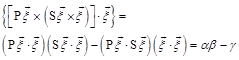
Lemma 1. ![]()
Proof. This formula is a corollary of that for the two-fold vector product. Indeed, according to the two-fold vector product formula
![]() . Taking a scalar product of both the given equality sides with
. Taking a scalar product of both the given equality sides with ![]() we find that
we find that
Let us derive differential equations for ![]() and
and ![]() . To do this let us compute the material derivatives of
. To do this let us compute the material derivatives of ![]() and
and ![]() .Keeping in mind that
.Keeping in mind that ![]()
![]()
![]() and
and ![]() , we obtain, on one hand, that
, we obtain, on one hand, that
and, on the other hand, that
Hence
![]() (3)
(3)
Similarly, we find, on one hand, that
![]() and, on the other hand, that
and, on the other hand, that
Hence
![]() (4)
(4)
Substituting ![]() instead of
instead of ![]() in Eq. (4) and subtracting Eq.(3) from the obtained equality term-wise we get finally the following differential equation
in Eq. (4) and subtracting Eq.(3) from the obtained equality term-wise we get finally the following differential equation
 (5)
(5)
Definition. Two non-zero vectors of ![]() and
and ![]() are said to be aligned perfectly if
are said to be aligned perfectly if ![]() ,i.e. when their vector (external) product is equal to zero.
,i.e. when their vector (external) product is equal to zero.
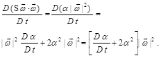
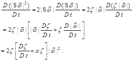
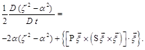
Considering Eq.(5) one can easily see that ![]() can be a solution to Eq.(5). Keeping in mind
can be a solution to Eq.(5). Keeping in mind ![]() one can easily find the differential equation for
one can easily find the differential equation for ![]() :
:
 (6)
(6)
Considering Eq.(6) one can easily see that ![]() can be solutions to Eq.(6). In particular, this is the case when
can be solutions to Eq.(6). In particular, this is the case when ![]() and
and ![]() are aligned perfectly. Indeed, by definition, the non-zero vectors
are aligned perfectly. Indeed, by definition, the non-zero vectors ![]() and
and ![]() are aligned perfectly provided that
are aligned perfectly provided that ![]() , i.e. when
, i.e. when ![]() .
.
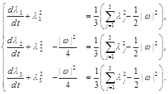
To define a notion of the restricted Euler equations, let us compute all
partial derivatives of the first equation of Eq.(1). In doing so we obtain the following equality
![]() (7)
(7)
Taking the symmetrical and antisymmetrical parts of Eq.(3) we find that
![]() . (8)
. (8)
In general the Hessian ![]() is the non-local non-isotropic matrix. Computing
is the non-local non-isotropic matrix. Computing
![]() of Eqs. (7, 8) we find that
of Eqs. (7, 8) we find that ![]() , where
, where ![]() is a trace of the matrix
is a trace of the matrix ![]() .
.
Definition. If to make violence and to assume ![]() to be local and isotropic of the kind
to be local and isotropic of the kind ![]() , we obtain then a model which is now called the "restricted Euler equations" [8].
, we obtain then a model which is now called the "restricted Euler equations" [8].
Here, the elliptic pressure constraint,![]() ,is concerned solely with the diagonal elements of
,is concerned solely with the diagonal elements of ![]() .
.
Let us study the restricted Euler equations. Since, for any ![]() and
and ![]() ,
, ![]() ,
,![]() is the eigenvector of
is the eigenvector of ![]() .
.
The latter implies in turn that![]() identically, for all
identically, for all ![]() and
and ![]() .1
.1
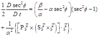
This leads to considerable simplification of Eqs.(5,6) which take the following form:
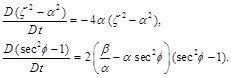 (9)
(9)
If to use the Lagrangian variable, we can then rewrite Eq. (9) legitimately as
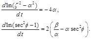 (10)
(10)
Integrating Eq. (10) we obtain two families of solutions of the kind
 (11)
(11)
where ![]()
![]()
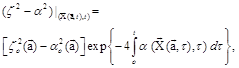
![]() It is evident from Eq.(11)that
It is evident from Eq.(11)that ![]() for
for ![]() provided
provided ![]() as well as
as well as ![]()
for ![]() provided
provided ![]() too. Thus we proved the following.
too. Thus we proved the following.
Proposition 1. Given the restricted Euler equations. If there is ![]() such that
such that ![]() are aligned perfectly, then
are aligned perfectly, then ![]() are aligned perfectly forever, for all admissible
are aligned perfectly forever, for all admissible ![]() .
.
Let ![]() be the eigenvectors of
be the eigenvectors of ![]() associated with its eigenvalues
associated with its eigenvalues ![]() There is a generally accepted convention respecting ordering of
There is a generally accepted convention respecting ordering of ![]() It is not assumed in what follows. It is not difficult to show that if
It is not assumed in what follows. It is not difficult to show that if ![]() is an eigenvector for
is an eigenvector for ![]() i.e., for example,
i.e., for example,![]() then, in the frame of
then, in the frame of ![]() the operators of
the operators of ![]() and
and ![]() take the following looks:
take the following looks:
In order to prove what is just aforesaid let us find now what is a matrix form of ![]() in the orthonormal frame of eigenvectors of
in the orthonormal frame of eigenvectors of ![]() provided that
provided that ![]() is one of the eigenvectors of
is one of the eigenvectors of ![]() .
.
Lemma 2. Given ![]() be an eigenvector for
be an eigenvector for ![]() associated with its eigenvalue
associated with its eigenvalue ![]() . Then
. Then ![]() ,
,![]() are the very same for
are the very same for ![]() .
.
Lemma 3. Let ![]() be an eigenvector for
be an eigenvector for ![]() or
or ![]() .Then
.Then ![]() is the same for
is the same for ![]() .
.
Proof of the lemmas. First of all notice that ![]() Therefore, due to the definition of
Therefore, due to the definition of ![]() , if
, if ![]() is the eigenvector for
is the eigenvector for ![]() associated with its eigenvalue
associated with its eigenvalue ![]() , the one is the eigenvector for
, the one is the eigenvector for ![]() associated with the very same eigenvalue and vice versa.
associated with the very same eigenvalue and vice versa.
Remark. Keeping in mind that the eigenvalues of ![]() all are real we can see that if
all are real we can see that if ![]() is the eigenvector for
is the eigenvector for ![]() or
or![]() , then one is associated to the mutual real eigenvalue of
, then one is associated to the mutual real eigenvalue of ![]() and
and![]() .
.
It can be easily to check that there is a rotation symmetry of solutions to the restricted Euler equations in the sense of if ![]() is a solution pair to the restricted Euler equations, then
is a solution pair to the restricted Euler equations, then ![]()
![]() is the same pair for any real orthogonal matrix
is the same pair for any real orthogonal matrix ![]() (i.e. such that
(i.e. such that ![]() ). It is well-known also (see, e.g., [9], p. 258) that any real symmetric matrix is orthogonally similar to the diagonal one. Therefore, without loss of generality, we can assume that the aforementioned coordinate transformation is made from the very beginning and the Cartesian coordinates are chosen in such a manner that they coincides accurate to translation on some constant vector with the eigenvector frame of
). It is well-known also (see, e.g., [9], p. 258) that any real symmetric matrix is orthogonally similar to the diagonal one. Therefore, without loss of generality, we can assume that the aforementioned coordinate transformation is made from the very beginning and the Cartesian coordinates are chosen in such a manner that they coincides accurate to translation on some constant vector with the eigenvector frame of ![]() and in doing so the vorticity direction
and in doing so the vorticity direction ![]() coincides, for instance, with that of the
coincides, for instance, with that of the ![]() -axis, i.e. that
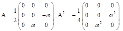
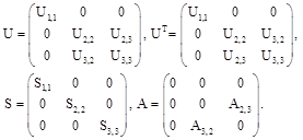
-axis, i.e. that ![]() It is evident that, in the given frame,
It is evident that, in the given frame,![]() is the diagonal matrix whose non-zero entries are
is the diagonal matrix whose non-zero entries are ![]() Keeping in mind this and that
Keeping in mind this and that ![]() one can specify better entries of
one can specify better entries of ![]() in such a manner:
in such a manner: ![]() Since
Since ![]() is the eigenvector for
is the eigenvector for ![]() and
and![]() , we find, as a corollary, that
, we find, as a corollary, that ![]() and also that
and also that ![]() Therefore, in the frame under consideration, the matrices
Therefore, in the frame under consideration, the matrices ![]() should have in general the following look:
should have in general the following look:
Remark. We notice attention that although the matrices ![]() and
and![]() have a canonical look in the eigenvector frame of
have a canonical look in the eigenvector frame of ![]() , the ones are not normal. It can be easily checked if to compute products
, the ones are not normal. It can be easily checked if to compute products ![]() and to compare them then.
and to compare them then.
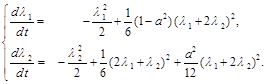
Applying to ![]() methods used in [5] for studying of behavior of eigenvalues of
methods used in [5] for studying of behavior of eigenvalues of ![]() one can show by the very same manner as it is done in [5] that, in the case
one can show by the very same manner as it is done in [5] that, in the case ![]() dynamics of
dynamics of ![]() are described by the next equations:
are described by the next equations:
 (12)
(12)
Really, keeping in mind that ![]() , we can rewrite the first equation of Eq.(8)in such a manner:
, we can rewrite the first equation of Eq.(8)in such a manner:
![]() (13)
(13)
Remark. It is worth to give attention that Eq.(12) is distinctly
distinguished from that presented in [5,7] (see, for example, Eq.(6.2)[5] or Eq.(1.6)[7]). This difference occurs because of different objects under study: we consider the strain matrix ![]() while the authors of [5-7] examine the velocity gradient matrix
while the authors of [5-7] examine the velocity gradient matrix ![]() .
.
Proposition 2. Given the restricted Euler equations. If ![]() i.e. is the eigenvector for
i.e. is the eigenvector for ![]() associated with its eigenvalue
associated with its eigenvalue![]() , then the dynamics of
, then the dynamics of ![]() is governed by Eq.(12).
is governed by Eq.(12).
Proof. ![]() by definition. Differentiating this relation with respect to $t$ we find
by definition. Differentiating this relation with respect to $t$ we find ![]() Computing a scalar product of the given equality terms with
Computing a scalar product of the given equality terms with ![]() we obtain
we obtain ![]() . Differentiation of the same relation with respect to
. Differentiation of the same relation with respect to ![]() leads to
leads to ![]()
Multiplying this equality by ![]() first and taking then a scalar product with
first and taking then a scalar product with ![]() we have
we have ![]() Therefore,
Therefore,![]()
Observing that ![]() and that
and that ![]() as well as
as well as ![]() and combining these facts with ones stated above one can easily see due to Eq.(13) that the proposition statement is valid in fact.
and combining these facts with ones stated above one can easily see due to Eq.(13) that the proposition statement is valid in fact.
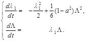
Subtracting the last equation of Eq.(12) from the previous one termwise we find after easy transformations that
![]()
Integrating this equation we obtain
![]() (14)
(14)
On the other hand, recalling that ![]() and taking into account that
and taking into account that ![]() is the eigenvector for
is the eigenvector for ![]() associated with its eigenvalue
associated with its eigenvalue ![]() we see that
we see that ![]() . Using the Lagrangian variables converts it to the following
. Using the Lagrangian variables converts it to the following ![]() . Integrating of the latter gives
. Integrating of the latter gives
![]() (15)
(15)
Comparing Eqs.(14-15) one can see that
![]() . (16)
. (16)
Thus, in the case under consideration, dynamics of ![]() is the very same as that of difference of the matrix
is the very same as that of difference of the matrix ![]() eigenvalues which are not associated with
eigenvalues which are not associated with ![]() Substituting
Substituting ![]() instead of
instead of ![]() in Eq.(16) we find that
in Eq.(16) we find that
![]()
If to substitute the expressions of ![]() and
and ![]() involving
involving ![]() and
and ![]() in the first two equations of Eq.(12) only we obtain the next ones:
in the first two equations of Eq.(12) only we obtain the next ones:
 (17)
(17)
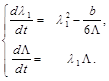
When ![]() we can easily integrate the first equation of Eq.(17).
we can easily integrate the first equation of Eq.(17).
![]() (18)
(18)
We see that ![]() does not blow up for a finite time provided
does not blow up for a finite time provided ![]() and blows up at
and blows up at ![]() for any
for any ![]() . In doing so
. In doing so ![]() as
as
![]() . But what is interesting is
. But what is interesting is ![]() as
as ![]() .
.
Unfortunately, we can say nothing respecting whether such the behavior of ![]() contradicts to the celebrated BKM criterion [10] or not because the latter involves norms of
contradicts to the celebrated BKM criterion [10] or not because the latter involves norms of ![]() in the Sobolev space
in the Sobolev space ![]() and integrals with respect to time of those of
and integrals with respect to time of those of ![]() in the
in the ![]() space. Let us pay attention also to that
space. Let us pay attention also to that ![]() enlarges at infinity as
enlarges at infinity as ![]() although the difference
although the difference ![]() remains bounded up to time
remains bounded up to time ![]() . It is a corollary of
. It is a corollary of ![]() and the behavior of
and the behavior of ![]() stated above.
stated above.
Let us change a variable setting ![]() In doing so Eq.(17) takes the look
In doing so Eq.(17) takes the look
 (19)
(19)
Multiplying the former of Eq.(19) on the latter crosswise we obtain ![]() or, otherwise,
or, otherwise, ![]()
Therefore, there is a first integral
![]() (20)
(20)
where ![]() We take into account here that
We take into account here that ![]() and
and ![]() Solving Eq.(20) we find
Solving Eq.(20) we find ![]()
Substituting the given expression in Eq.(19) we obtain
 (21)
(21)
When ![]() we can easily integrate the first equation of Eq.(21).
we can easily integrate the first equation of Eq.(21).
Namely: ![]() We see that
We see that ![]() has no blow up for a finite time provided
has no blow up for a finite time provided ![]() and blows up at
and blows up at ![]() for any
for any ![]() . The same takes place for
. The same takes place for ![]() and
and ![]() too.
too.
What is the aforesaid can be summarized in view of the following.
Proposition 3. Given the restricted Euler equations. If there is
![]() such that
such that ![]() are aligned perfectly, then, for certain initial conditions, the eigenvalues of
are aligned perfectly, then, for certain initial conditions, the eigenvalues of ![]() lose their initial smoothness for a finite time by means of the so-called "finite-time blow up". As for the vorticity, it can as undergo the similar blow up at the same time as cannot.
lose their initial smoothness for a finite time by means of the so-called "finite-time blow up". As for the vorticity, it can as undergo the similar blow up at the same time as cannot.
Thus, an approach based on studying of the perfect alignment between the vorticity vector and the strain matrix eigenvectors permits us to deepen some results in [5] and to specify scenarios of the finite time blow ups of the restricted Euler equations solutions. To be more precise, Lemmas 6.1 - 6.2 [5] inform that the aforesaid solutions blow up at a finite time for almost all initial gradient matrix ![]() But they say nothing how it occurs and what happens at the blow up time. The principal results presented above describe two concrete very different scenarios of the aforesaid blow ups.
But they say nothing how it occurs and what happens at the blow up time. The principal results presented above describe two concrete very different scenarios of the aforesaid blow ups.
Remark. We would like to attract a reader attention once more to that a
situation when the eigenvalues of ![]() blow up for a finite time and in doing so the vorticity does not is, generally speaking, unexpected if to take into account the celebrated BKM criterion for solutions to the (genuine!) Euler equations to blow up at a finite time.
blow up for a finite time and in doing so the vorticity does not is, generally speaking, unexpected if to take into account the celebrated BKM criterion for solutions to the (genuine!) Euler equations to blow up at a finite time.
4. Conclusions
Summarizing all what is the aforesaid respecting the blow ups of solutions to the restricted Euler equations we can infer that their properties differ from those of solutions to the genuine Euler equations very essentially. Really, as is just marked above there are parameter data and initial conditions such that the eigenvalues of the strain matrix ![]() for the restricted Euler equations blow up for a finite time and in doing so their vorticity does not and vice versa. However, such kind a behavior is completely not possible for the Euler equations because, as it was shown by G.Ponce in [12], a finite-time blow up of the Euler equations vorticity
for the restricted Euler equations blow up for a finite time and in doing so their vorticity does not and vice versa. However, such kind a behavior is completely not possible for the Euler equations because, as it was shown by G.Ponce in [12], a finite-time blow up of the Euler equations vorticity ![]() accompanies the very same one of the strain matrix
accompanies the very same one of the strain matrix ![]() and, as a corollary, of its eigenvalues and vice versa. Therefore, the model under study cannot be considered as suitable one for recognizing and study of properties inherent to the Euler equations solutions. Nevertheless, in itself it is of considerable interest because exhibits unexpected features.
and, as a corollary, of its eigenvalues and vice versa. Therefore, the model under study cannot be considered as suitable one for recognizing and study of properties inherent to the Euler equations solutions. Nevertheless, in itself it is of considerable interest because exhibits unexpected features.
References
- Viellefosse P.: Local interaction between vorticity and shear in aperfect incompressible fluid. J. Phys. Paris. vol.43 (1982), 837-842.
- Viellefosse P.: Internal motion of a small element of fluid in aninviscid flow. Physica A. vol.125 (1984), 150-162.
- Novikov E.A.: Internal dynamics of flows and formation of singularities. Fluid Dynam. Res. vol.6 (1990), 79-89.
- Cantwell B.J.: Exact solution of a restricted Euler equation for thevelocity gradient tensor. Phys. Fluids. vol.4, no. 4 (1992), 782-793.
- Liu H. and Tadmor E.: Spectral dynamics of the velocity gradient field in restricted flows. Commun. Math. Phys. 228 (2002), 435-466.
- Liu H. and Tadmor E.: Critical thresholds in 2D restricted Euler-Poisson equations. SIAM J. Appl. Math., vol. 63, no. 6 (2003), 1889-1910.
- Liu H., Tadmor E. and Wei D.: Global regularity of the 4D restrictedEuler equations. Physica D (2009), doi: 10.1016/j.phesd.2009.07.009.
- Gibbon J.D.: The three-dimensional Euler equations: Where do we stand? Physica D. vol. 237 (2008), 1894-1904.
- Gantmakher F.R., Theory of Matrices, 3th edition, "Nauka" PublishingHouse, Moscow, 1967, 575 p. (in Russian).
- Beale J.T., Kato T. and Majda A.: Remarks on the breakdown of smoothsolutions for 3-D Euler equtions. Commun. Math. Phys. 94 (1984), 61-66.
- Dobrynskii V.A.: Perfect vector alignment of the vorticity and thevortex stretching is one forever. Forum Mathematicum (2011, september), DOI~10.1515~/FORM.2011.149, 13 pp.
- Ponce G.: Remarks on a paper by J.T.Beale, T.Kato and A.Majda.Commun. Math. Phys. 98 (1985), 349-353.
Footnotes
1 Indeed, taking into account that according to the two-fold vector product formula, what is the aforesaid can be reformulated with aid of the Lagrangian variables as follows: for all and ,


