
International Journal of Mathematics and Computational Science, Vol. 1, No. 5, October 2015 Publish Date: Jul. 23, 2015 Pages: 295-302
Groundwater Flow Transfixion of Deep Heat Reservoir and Its Influence on Temperature Field
Aidi Huo1, 2, 3, *, Zhiyuang Ma1, Shiyan Guo4, Yalei Du1, Fengmei Su1
1School of Environmental Science & Engineering, Chang’an University, Xi’an, Shaanxi, P.R. China
2Key Laboratories of Environmental Protection & Pollution and Remediation of Water and Soil of Shaanxi Province, Xi’an, P.R. China
3State Key Laboratory of Simulation and Regulation of Water Cycle in River Basin, China Institute of Water Resources and Hydropower Research, Beijing, P.R. China
4Sinopec Green Energy Geothermal Development Co., Ltd, Xianyang, P.R. China
Abstract
The distance between production and injection wells, distribution of wells and operation models of the pump system are the key determining factors of the system work efficiency. A new concept of flow transfixion is suggested by analyzing the general features of an aquifer. A couple numerical models of groundwater flow and heat transferring were established based on the basic theory of water-heat transferring in the aquifer. The interaction between flow and heat transfixions, and its significance to practical engineering were also analyzed. And then numerical analysis of the flow field and the temperature field for the pump system in one community of Xianyang City shows that the main factor of the formation of flow transfixion is hydraulic gradient, namely, the hydraulic gradient can be used to judge quantitatively whether the flow transfixion takes place or not. The effect of the injecting and pumping rate (Q) to the flow transfixion shows that the shorter occurrence time of flow transfixion, the more of the value of Q, and it is easier to occur flow transfixion for more of Q, and then to lead to occurrence of heat transfixion. In practical engineering, the occurrence of heat transfixion can be reduced by reducing the value of Q, and by increasing spacing of injecting and pumping wells.
Keywords
Production-Injection Well System, Thermal Energy Storage of Aquifer, Enforce Convection, Flow Transfixion, Heat Transfixion
Received: June 28, 2015
Accepted: July 11, 2015
Published online: July 23, 2015
@ 2015 The Authors. Published by American Institute of Science. This Open Access article is under the CC BY-NC license. http://creativecommons.org/licenses/by-nc/4.0/
Contents
1. Introduction 2. Materials and Methods 2.1. The Couple Numerical Model of Underground Heat Reservoir 2.2. The Study Area and Boundary Conditions 3. Simulation Results and Analysis 3.1. Simulation Analysis of Connected Water 3.2. Analysis of the Influence That Flow Transfixion’s Production on Temperature Field 4. Conclusions Acknowledgement
1. Introduction
Under the background of energy consumption and serious environmental pollution, the underground deep heat reservoir with its advantages of clean and pollution-free renewable water, has quickly become the new energy source that every country promotes actively. Groundwater, as low heat source, solves the problem of refrigeration in summer and heating in winter by constructing production and injection wells system (PWIS) to extract the amount of heat or cold in groundwater.
The main problem during developing and utilizing the geothermic is that geothermal reservoirs temperature and pressure decreased when production and time increased (Chen 1998). At the same time the discharge of geothermal water caused thermal pollution to the environment (Shen and Zhang 1998). Now, we think that injection can effectively solve the problems which geothermal exploitation and utilization creative. So the injection and exploitation of geothermal are popularized and applicated in the global scope. The number of wells are rapidly increasing because wells can exploited geothermal energy. Recently, the research about heat reservoir and injection was also started all over the world (Tenma et al. 2003).
In the related research, the ground aquifer was treated as energy storage layer to study the changes of the internal temperature field. The law of groundwater heat conduction and the mechanism analysis of underground aquifer’s heat exchange had many achievements (Ma et al. 2005; Ni and Ma 2006; Zhu et al. 2011). Paksoy et al. (2004) put the pumping well’s water level falling and injection well’s water level rising as constraint conditions. Thought modeling they analyzed production and injection well’s minimum separation in the context that "heat transfixion" did not occur. Tenmaa conducted the software FEHM to establish the ideal model of wells(Ni and Ma 2006). They carried on comparison and analysis by simulating the location’s layout plan, operation time, injection amount, mining method, pipe length and some other working conditions. Zhang et al. (1999) did some research about groundwater temperature change trend under the condition of the same well. The main influencing factors included cold and hot load, aquifer parameters’ choosing, thermal diffusion coefficient, etc. On the basis of HST3D which USGS developed to simulate heat transferring and solute transportation, Zhang et al. (1999) also set up a numerical model of deep well injection in underground water source heat pump system. They conducted numerical simulations on the changes in temperature field and underground water level for a long time and verified model’s functional and adaptability.
There already were some reports on the work about separate heat conduction, heat transfixion, enforce convection and so on. But there was little literature about transfixion problems around energy storage well and the relationship between flow transfixion and heat transfixion until today when the occurrence of flow transfixion was determined by temperature field’s distribution in energy storage layer and the occurrence of heat transfixion. To know the distribution of low field and temperature field in energy storage layer clearly, to set pumping well spacing reasonably, to improve the efficiency of underground thermal storage , and to prevent the occurrence of thermal transfixion, it’s necessary to do some research about the changes of fluid field and temperature field in an aquifer on different injection parameters to predict the distribution state of underground "cold and hot reservoir" and finally provide reliable basis for engineering design of an aquifer. Based on the groundwater flow model and heat transport model to analyze the mechanism of groundwater appearing flow transfixion and the influence it brings to thermal transfixion, this paper puts the water heat pump engineering in a residential area of Xianyang city, Shaanxi province for an example, then we can get the approach of making reasonable distance between production and injection wells and provide scientific foundation for the reasonable design of the PIWS.
2. Materials and Methods
2.1. The Couple Numerical Model of Underground Heat Reservoir
Research has been conducted on thermal-hydrological coupling model of aquifer energy migrated (Zhao et al. 2009; Zhang et al. 2006; Yuan et al. 2009). The level structure, heterogeneity and anisotropy are used to confine the aquifer commonly in the three-dimensional unsteady flow system. In this kind of premise, deformation of the geological structure was mainly in the vertical direction and kept approximate constant in the horizontal direction. At the same time, aquifer porosity was variable while assuming that the density of water was constant.
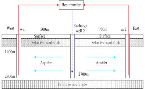
Fig. 1. The Conceptual model diagram of pumping model.
Figure 1 is the conceptual model diagram of pumping model (wr1’s not recharged). For production and injection wells, we can use this mode during the seasonal alternation.
For heterogeneous and anisotropic confined aquifer, while production and injection wells running, the fundamental equations, which describe porous medium three dimensional non steady flows and the heat transport, are as following:
![]() (1)
(1)
![]() (2)
(2)
![]() (3)
(3)
where, ![]() —The seepage velocity component in spatial coordinates, m /s; n —Effective porosity, %;
—The seepage velocity component in spatial coordinates, m /s; n —Effective porosity, %; ![]() —Osmotic coefficient, m /s;
—Osmotic coefficient, m /s; ![]() —Waterhead, m;
—Waterhead, m; ![]() — Fluid density, kg /m3;
— Fluid density, kg /m3; ![]() ,
,![]() —Porous media\The fluid heat capacity. J /m3°C;
—Porous media\The fluid heat capacity. J /m3°C; ![]() — Dispersion coefficient, J /(m d°C ); T —Temperature, °C; t —Time, s; µe-Elastic storage coefficient, dimensionless; K-Osmotic coefficient, m/d; M- Aquifer thickness, m; ε-Vertical supply intensity, m3/(d.m2)= m/d;
— Dispersion coefficient, J /(m d°C ); T —Temperature, °C; t —Time, s; µe-Elastic storage coefficient, dimensionless; K-Osmotic coefficient, m/d; M- Aquifer thickness, m; ε-Vertical supply intensity, m3/(d.m2)= m/d; ![]() : Storage coefficient.
: Storage coefficient.
2.2. The Study Area and Boundary Conditions
The study area Located in the central part of Shaanxi province, China, Xianyang city is about 30 kilometers (19 miles) northwest of Xi’an with the Weihe River immediately to the south(Xi et al. 2014; Li et al. 2013). We analyzed PIWS with this model, and simulated calculations on its groundwater flow field by Modflow software in study areas. We got its essential information and then got heat affected zone by simulation analysis, and finally got hydrothermal coupling relationship in this area which provided reasonable gist for engineering practice there.
The target area was a square area of 2000 m × 2000 m. There were 5 wells in the middle (Figure 2). The simulation area was located in River’s first level region, so it was unconsolidated aquifer formed by deposition. It belonged to the same level pumping and the distance was small. According to the supplying structure of pumping and observation wells, we knew that each well had similar lithology and its adjacent rock’s lithology variation was small. So the rocks in the study area could be summarized as horizontal extension. Pumping well mesh only occurred in the shallow confined aquifer under 1400 m. It mainly simulated the hydraulic distribution of a confined aquifer. So the rocks above 1400 m could be summarized as aquitard. Between 1400 m to 2800 m, lithology mostly was coarse sand and coarse sand, which were aquifer. There were clay and silt below 2800 m and it could be seen as aquitard.
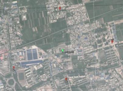
Fig. 2. The location of study area.
Above all, there were three layers in vertical direction. The total depth was 3000 m. From top-down: 0 to 1400 m below ground was aquitard, mainly was Sanmen group and Zhangjiapo group; 1400 to 2700 m was first shallow confined aquifer, mainly was Lantianba group; 2700 to 3000 m was aquitard, mainly was Jianxintong; Under 3000 m was aquifuge. This research was divided into two experiments: one was pumping and injection test, the other was injection temperature measurement test. Pumping rate was 1883 m3/d. Temperature was 55°C. Running time was 120 d in one year. Reinjection water temperature was 36°C. Reinjection time was 120d. Recharge volume was 2890 m3/d.
Table 1. Parameter values.
| Parameter name | Meaning | Parameter values |
| H | Depth(m) | 1400-2700 |
| Kx | Vertical permeability coefficient(m/d) | 0.44 |
| Ky | Lateral coefficient of permeability(m/d) | 0.44 |
| Kz | Vertical permeabilitjy coefficient(m/d) | 0.044 |
| Sy | Specific yield | 0.26 |
| Ss | Storage coefficient | le-5 |
| Kd | Distribution coefficient(L/mg) | 0.00003 |
| D | Dispersity(m) | 10 |
| n | Active porosity | 0.15 |
|
| Total porosity | 0.35 |
| R | Recharge intensity (mm/yr) | 0 |
| ET | Evapotranspiration | 0 |
|
| Evaporation critical depth(m) | 0 |
| Long.Disperivity(M) | 10 | |
| Horiz./Long.Dispersivity | 0.1 | |
| Vert./Long.Dispersivity | 0.01 |
In analog computation, we selected the simulation parameters in the region combined with its geology of aquifer and hydrogeological condition. We set aquifer as heterogeneity and anisotropy. The ranges of values for each parameter used in this study are reported in Table 1, in which the main parameters, H, K, Sy, Ss, Kd, D, n, and ![]() , comes from the report of well completion. Further data, such as R,ET, and Hk, on these simulations are available in the supporting information data set.
, comes from the report of well completion. Further data, such as R,ET, and Hk, on these simulations are available in the supporting information data set.
3. Simulation Results and Analysis
Assume a cycle term of water extracting and filling was one year. It could be divided into two stages: The first stage for heating was 4 months (2880 h) while intermittent period was 2 months (1440 h); the second stage for cooling was 4 months (2880 h) while intermittent period was 2 months (1440 h). After one stage, switch the position of pumping well and injection well. In this way, the influence of heat transport could be reduced and the thermal penetration probability of underground energy storage layer could be lowered. It could also increase the energy utilization efficiency of underground energy storage layer to prevent recharge coefficient in underground energy storage layer from reduced enegy which was caused by physical, chemical and biological factors.
3.1. Simulation Analysis of Connected Water
|
|
|
|
| a. groundwater-table contour map in Pumping well and Injection well operated 1.6 days | b. groundwater-table contour map in Pumping well and Injection well operated 2 days | c. groundwater-table contour map in Pumping well and Injection well operated 15 days |
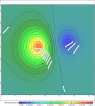
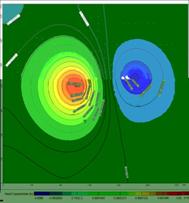
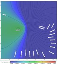
Fig. 3. The simulation area of groundwater-table contour map in Pumping well and Injection well operated 1.6,2 and 15 days.
Fig. 3 shows the simulation area of groundwater-table contour map in pumping well and injection well operated 1.6, 2 and 15 days. We can see the change of groundwater movement. In the initial time of operation, natural flow field was less affected by pumping and injection (Fig. 3a). The underground water level had obvious changes within the range of 2 m. As the pumping time extended, the influence of pumping well and injection well increased. Fig.3b shows the groundwater-table contour map in pumping well and injection well operated 2 days. The influence of pumping well and injection well was obviously increased. The underground water level had obvious changes. Since then it changed little. It showed that after 2 days, the groundwater flow field formed new steady flow field with the joint action of water pumping and irrigation and source sink term of boundary. After 15 days, the connection of the flow field occurred between production and injection well. The groundwater stored in the irrigation wells aquifer had been made as the amount of production and injection increased. So the water which the pumping well injected into the aquifer began to spread to the aquifer around the irrigation well. In the direction of the pumping well, water continuously came into the influence of the pumping well. So groundwater which injection water pumped into the aquifer began to be pumped by the pumping well (Fig.3c).
Fig.4 shows the change curve of head between pumping and injection wells in 0.41d、0.76d、1.6d、2.0d and 15d. The hydraulic slopes were 0.0004113、0.000791、0.001448、0.001669 and 0.00138m. After 1.6d, the changes of hydraulic slope were very small which could be disregarded. When hydraulic slope kept constant, the energy storage laminar flow field incurred new stabilization, namely flow transfixion. It was the same with Fig.3. So we could quantificationally judge whether flow transfixion happened or not by hydraulic slope and then get the concept of flow transfixion, namely that underground flow field incurred stable seepage phenomenon with the forced convection of the pumping and injection wells, and the water injected by the injection well was pumped out.
We simulated the underground water level amplitude in different extraction volume and found that the constant time of underground water lever changed as the extraction volume changed. And when pumping and extraction volume increased, underground changed obviously affected by pumping and injection wells and the constant time decreased. It showed that the time of flow transfixion was shorten mainly because that underground water occurred forced convection’s reinforce with pumping and injection water to ignore the function of natural flow field. A new stable seepage flow field formed in a certain time with the influence of forced convection. When it was formed, flow transfixion would also occur.
Fig.6 shows that when the distance of wells was different, the change curve of water head and time of the observation well was not obvious. But when the distance was 68 to 120 m, the water head of injection well rise in the early and then decline with the influence of the pumping well. When the distance was 140m or any farther, the head didn’t change over time. So it was beyond the influence scope of the pumping well and we could use 140 m as the upper limit of reasonable distance.
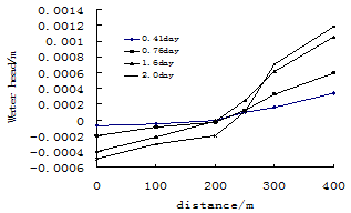
Fig. 4. The change curve of water head at differet locations during 0.41,0.76,1.6,and 2.0 days.
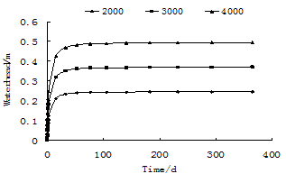
Fig. 5. The change curve of water head of observation wells with different quantity of water:2000,3000,4000m3/d.
Fig.5 shows the change curve of the water head and time of injection and pumping wells with different distance between observation and recharge wells. It was 300 m far from injection wells. When extraction volume was 2000m3/d,the time when underground water formed new steady fluid field was about 600 h. But when it came to 5000m3/d,the time decreased to about 400h, which could explain that the time of flow transfixion decreased with extraction volume increasing. When PIWS had run over the water in a cycle, the groundwater’s water level amplitude, constant time and the alteration of the temperature field in different distance could be simulated. So the distance of pumping and injection wells could be confirmed.
3.2. Analysis of the Influence That Flow Transfixion’s Production on Temperature Field
Recharge water temperature had some differences with the original aquifer temperature. Under the function of heat conduction and convection, the temperature of the water-fronts of injection wells would make the outlet water temperature of the pumping well nearby go up or down in different degrees, which was often called heat transfixion. To make the influence scope of temperature field in injection well least and prevent it from forming heat transfixion, it was necessary to do research on the difference of the influence scope of temperature field in different quantity of water recharge.
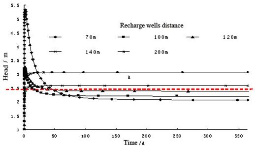
Fig. 6. The change curve of head and time of injection and pumping wells with different distance between observations well and recharge well.
Table 2. Calculated velocities of groundwater flow under different quantity of water.
| Q/(m3/d) | △H/m | I | v/(m/d) |
| 2000 | 0.25 | 0.000673 | 3.13 |
| 3000 | 0.37 | 0.001013 | 3.44 |
| 4000 | 0.49 | 0.001353 | 3.75 |
| 5000 | 0.58 | 0.001589 | 4.17 |
Table 2 shows the calculated velocities of groundwater flow under different quantity of water. The larger the quantity of water recharge was, the bigger the hydraulic gradient and seepage flow velocity were. According to the research, when energy abstraction system was running, the main way of heat transfer near the pumping and injection wells was convective heat transfer. Convective heat transfer mainly depended on groundwater flow velocity (Zhang et al. 2006). So the larger the quantity of water recharge was, the faster the velocity of groundwater flows was, while convection heat transfer in unit time was larger and the temperature of pumping well changed faster.
To draw the influence scope of temperature in aquifer better, we assume that the area which the temperature of aquifer decreased at least 2°C was the influenced scope by the recharge of the injection well. Fig.7 shows that the maximum value (the influence distance in the direction of the flow) of influence scope under 4 conditions was increased with time. In the same quantity of water recharge, the influence scope expanded as time increased. During the same time, the bigger the quantity of water recharge in unit time was, the larger the influence scope of it was.
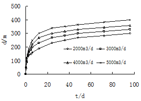
Fig. 7. The change curve of influence of temperature field and time with different quantity of water.
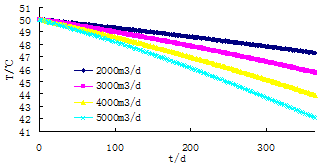
Fig. 8. The change curve of temperature and time of observations well with different quantity of water.
Under the working condition of 4000m3/h, the influence scope expanded to the pumping well after 300 d, namely thermal transfixion occurs. It differs by about 300 d from the occurrence time of flow transfixion under the same quantity of water recharge. This explained that thermal transfixion occurred after flow transfixion had happened for a while. Heat migration happened associated with the flow field’s connection, which could also be explained by other flow. So we could control thermal transfixion by control flow transfixion. Compare the influence scope of heat in different quantity of water recharge and without pumping well (no forced convection), we could knew that it changed little without forced convection. And it decreased as time changed, which was shown in Fig.8. During 700 h, the quantity of water recharge was 2000 m3/h. The influence scope of the temperature field had reached 100 m, which was only 50 m in the condition of none forced convection. So the forced convection of water pumping had great influence on the spread of the geothermal field.
To draw the influence scope of temperature in aquifer better, we assume that the area that the temperature of aquifer decreased at least 2°C was the area that was influenced by recharge, namely heat transfixion. The Fig. 9 shows the change curve of temperature and time with different distance between observation and recharge wells. The larger the distance is, the longer the time to occur heat transfixion is. And the range ability of pumping temperature would be smaller. When it came to the 5th year, the reasonable distance lower limit was 100 m in the premise that heat transfixion would not happen. Combined with the influence scope above, we could know the reasonable distance was 100m-140m in this study limited conditions.
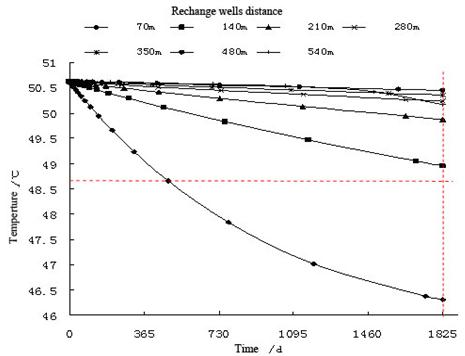
Fig. 9. The change curve of temperature and time with different distance between observations well and recharge well.
4. Conclusions
With combining the water flow numerical model of the ground aquifer and the numerical model of energy storage, this paper simulates the fluid field flow and temperature field in underground water to judge the flow transfixion with the changes of the hydraulic gradient. The conclusions are as follows:
(1) The coupling thermal-hydrological model was used to simulate the worksite in Xianyang City, Shaanxi province. The results show that it can be used to accurately and truly simulate the distribution of the groundwater flow and temperature fields in the actual situation.
(2) It provides the concept of the critical value of flow transfixion and gives quantitative judgment. When hydraulic gradient is constant, the new stability flow field occurs in energy storage laminar, that is the critical value of flow transfixion.
(3) With the constant distance between the pumping and injection wells, when the heat pumps works for a long time there will occur flow transfixion in the groundwater flow field. The larger the quantity is, the shorter the time of flow transfixion is.
(4) When the system is running 5y, the most reasonable distance is 100 m to 140 m in the premise that heat transfixion would not happen.
Pumping and injecting water heavily easily lead to flow transfixion and then thermal transfixion, which against the use of energy in practical engineering. To narrow the influence scope of heat in pumping well, we should reduce the water output and increase the distance between pumping and injection wells if possible. The position of pumping and injection wells could be adjusted while they have running for a cycle to reduce the influence scope of the heat affection.
Acknowledgement
The authors would like to acknowledge graduate students: Zhihan Yun, Lei Zhen, Dan Xu and huiJv Zheng from school of Environmental Science & Engineering in helping collecting the site data, Kara Cosentino from the University of Nebraska-Lincoln for helping correcting the English express. The authors also wish to express thanks to the Open Research Fund of State Key Laboratory of Simulation and Regulation of Water Cycle in River Basin (China Institute of Water Resources and Hydropower Research), Grant NO:IWHR-SKL-201510.
References
- Chen Z (1998) Modeling water _rock interaction of geothermal reinjection in the tanggu low_temperature field, Tianjin. Earth Science: Journal of China University of Geosciences 23 (5):513-518. (in Chinese, with English abstract)
- Li Y, Huo A, Liu R, Chen S,Wang X, Li J (2013) Water resources responses to climate changes in Xi’an Heihe River Basin based on SWAT model. Journal of Water Resources Research,2:301-308
- Ma J, Wang M, Dai B (2005) Research on aquifer's thermal energy storage and analysis of its different processes. Journal of North China Electrie Power University 31 (6):58-60.(in Chinese, with English abstract)
- Ni L, Ma Z (2006) Effect of Aquifer Parameters on Groundwater Heat Pump with Pumping and Recharging in Same Well. Journal of Tianjin University 39 (2.(in Chinese, with English abstract))
- Paksoy H, Gürbüz Z, Turgut B, Dikici D, Evliya H (2004) Aquifer thermal storage (ATES) for air-conditioning of a supermarket in Turkey. Renewable Energy 29 (12):1991-1996
- Shen J, Zhang G (1998) Environmental Protection and Environmental Impact of Geothermal Development and Utilization. Bullet in of the Chinese Academy of Geological Sciences 19 (4):402-408.(in Chinese, with English abstract)
- Tenma N, Yasukawa K, Zyvoloski G (2003) Model study of the thermal storage system by FEHM code. Geothermics 32 (4):603-607
- Xi D, Zhang S-Y, He Q-L, Chen L, Zhang J, Huo A-D (2014) A Coupled Model Simulation and Application of Swat-Modflow Based on the Technology of GPR. Journal of Water Resources Research 2014:301-308.(in China, with English abstract)
- Yuan j, Wang R, Yuan D (2009) Effects of Well Pair Distance on Pumping Temperature of Storage Exploiting in the Aquifer of Water. source Heat Pump. Building Science 25 (2):92-96.(in Chinese, with English abstract)
- Zhang Y, Wei J, Li Y, Li S (2006) Simulation of Changes in Geo-Temperature Field Due to Energy Abstraction from Underground Aquifers. Journal of Tianjin University 39 (8):(in Chinese, with English abstract)
- Zhang Y, Xue Y (1999) FIow equation with temperature variation and Its application in the aquifer thermal energy storage model. Geological review 45 (2):209-217.(in Chinese, with English abstract)
- Zhao J, Yan Z, Shao J, Cui Y, Liu X, Tian L (2009) Impact of pumping and injection modes on groundwater temperature in energy extraction area with regional flow. Journal of Hunan University of Science &Technology 2 (24):24-27.(in Chinese, with English abstract)
- Zhu H, Liu X, Yang F, Yang H, Wang X (2011) Analysis and study on geothermal reinjection test of deep groundwater in kaifeng. Journal of Henan Polytechnic University(Natural Science) 30 (2):215-219


