
International Journal of Mathematics and Computational Science, Vol. 1, No. 5, October 2015 Publish Date: Jun. 24, 2015 Pages: 242-249
Application of the GDQ Method to Vibration Analysis
Ramzy M. Abumandour1, *, M. H. Kamel2, M. M. Nassar2
1Basic Engineering Science Department, Faculty of Engineering, Menofia University, Shebin El-Kom, Menofia, Egypt
2Engineering Mathematics and Physics Department, Faculty of Engineering, Cairo University, Giza, Egypt
Abstract
This paper study the vibration analysis using the differential quadrature method (DQM) which has very wide applications in the field of structural vibration of various elements such as beams, plates, cylindrical shells and tanks. One of the most advantages of the DQM is its simple forms for nonlinear formulations. In this paper, the free vibration of uniform and non-uniform beams resting on fluid layer under axial force under three sets of boundary conditions, that is, simply–simply supported (S–S), clamped–clamped supported (C–C) and clamped–simply supported (C–S) were studied using the generalized differential quadrature (GDQ). The proposed approach directly substitutes the boundary conditions into the governing equations (SBCGE). The approach of directly SBCGE is presented to overcome the drawbacks of previous approaches in treating the boundary conditions. The non-dimensional natural frequency and the normalized mode shapes of uniform and non-uniform beams were obtained. Results show good agreement with the previous analytical solutions. The effect of the varying cross section area on the vibration was studied. This work reflects the power of the DQM in solving non-uniform problems.
Keywords
Uniform and Non-Uniform Beam, Vibration, Differential Quadrature Method
Received: April 9, 2015
Accepted: April 17, 2015
Published online: June 23, 2015
@ 2015 The Authors. Published by American Institute of Science. This Open Access article is under the CC BY-NC license. http://creativecommons.org/licenses/by-nc/4.0/
1. Introduction
Often, numerical approximation methods have to be sought to solve vibration problems due to the complexity of the problems. Classical techniques such as finite element and finite difference methods are well developed and well known. These methods can provide very accurate results by using a large number of grid points; thus they are computationally expensive. In a large number of cases, only a limited number of frequencies and mode shapes or a dynamic response at only a limited number of points is needed to be found. The DQM discretizes any derivative at a point by a weighted linear sum of functional values at its neighboring points. The key to DQM is the determination of weighting coefficients. Based on the idea of integral quadrature the DQM was first introduced by Richard Bellman [1,2]. Bellman et al. [2] suggested two methods to determine the weighting coefficients of the first order derivative. The first method used a simple function as test functions, the second method is similar to the first one with the exception that the coordinates of grid points should be chosen as the roots of the Nth order Legendre polynomial. Unfortunately, when the order of the algebraic equation system is large, its matrix is ill-conditioned. Thus it is very difficult to obtain the weighting coefficients for a large number of grid points using this method. To overcome the drawbacks, of the above methods, Quan and Chang [12], Wen and Yu [17] use Lagrange interpolation polynomials as test function, and then obtained explicit formulations to determine the weighting coefficient for the first and second order derivatives discretization. More generally, Shu and Richards [14], and Shu [15] present the generalized differential quadrature (GDQ). In GDQ, the weighting coefficients of the first derivative are determined by a simple algebraic formulation, and the weighting coefficient of the higher order derivatives are determined by a recurrence relationship. The major advantage of GDQ over DQ is its ease of the computation of the weighting coefficients without any restriction on the choice of grid points. The pioneer work for the application of the DQ method to the general area of structural mechanics. To solve these equations, the boundary conditions have to be implemented appropriately. For the case where there is only one boundary condition at each boundary. However, in some cases, there is more than one boundary conditions at each boundary, which could result in difficulties in the numerical implementation of the boundary conditions. One example is the solution of the flexural vibration analysis of a thin beam or a plate. The governing equation for bending of a thin beam or a plate is a fourth order differential equation with two boundary conditions at each boundary. The details of the DQ method can be found in reference [16].
2. Generalized Differential Quadrature Method
In order to overcome the deficiencies which appears in classical DQM, Bellman et al. [2], a generalized differential quadrature (GDQ), which was recently proposed by Shu and Richards [14,15] for solving partial differential equations in fluid mechanics, will be introduced and applied to solve some problems in vibration analysis. In order to find a simple algebraic expression for calculating the weighting coefficients without restricting the choice of grid meshes, Shu chose Lagrange interpolated polynomials as the set of tests functions g(x). Shu and Richards [14,15] gave a convenient and recurrent formula for determining the derivative weighting coefficients as follows:
![]()
![]()
![]()
![]() (1)
(1)
![]() , for
, for ![]() (2)
(2)
Equations (1) provide simple expressions for computing ![]() without any restriction in choice of the co-ordinates of the grid points xi. It is obvious that
without any restriction in choice of the co-ordinates of the grid points xi. It is obvious that ![]() can be easily calculated for i
can be easily calculated for i![]() j. The
j. The ![]() can be obtained from equation (2).
can be obtained from equation (2).
For the discretization of the second and higher order derivatives, the following linear constrained relationships are applied
![]() (3)
(3)
The recurrent formula for determining the derivative weighting coefficients as follows:
![]()
![]()
![]()
![]() (4)
(4)
![]() for
for ![]() (5)
(5)
where ![]() and
and ![]() are the weighting coefficients of the mth and the (m−1)th derivatives. The
are the weighting coefficients of the mth and the (m−1)th derivatives. The ![]() can be obtained from a relationship similar to equation (7).
can be obtained from a relationship similar to equation (7).
Thus equations (4) and (5) together with equation (1) and equation (2) give a convenient and general form for determining the weighting coefficients for the derivatives of orders one through ![]() .
.
3. GDQ Application
The method of GDQ is used to analyze the free vibration problems of uniform and non-uniform beams resting on fluid layer under axial force in this section. In this section will calculating the natural frequencies and drawing the mode shapes of uniform and non-uniform slender beams under three sets of boundary conditions, that is, simply–simply supported (S–S), clamped–clamped supported (C–C) and clamped–simply supported (C–S). The formulations and programming are shown to be very straightforward and simple. The boundary conditions are easy to be implemented.
Basic Equations
1. Fluid Back Pressure Equations
For an incompressible, irrotational, inviscid fluid of constant density γf the pressure of the fluid Pf(x,y,t) satisfies the following equation:
![]() (6)
(6)
where;
The contact conditions are:
![]() ,
, ![]() (7a)
(7a)
![]() ,
, ![]() (7b)
(7b)
The initial conditions are:
![]() (7c)
(7c)
The method of separation of variables is used to determine the fluid back pressure (Pf),
![]() (8)
(8)
Substituting equation (8) in equation (6) yields;
![]() (9)
(9)
where; ![]() is the fluid linear stiffness.
is the fluid linear stiffness.
2. Beam Equations
The governing equation of a Bernoulli–Euler beam in bending is given by:
![]()
![]() (10)
(10)
where EI is the beam’s flexural rigidity, ρA is the mass per unit length, L is the length of the beam and ![]() is the fluid back pressure.
is the fluid back pressure.
Normalizing the equation (10) then the non-dimensional governing equation of a Bernoulli-Euler beam of varying cross-section resting on fluid layer under axial force may be written as:
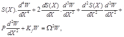 (11)
(11)
where the non-dimensional coefficients is;
![]()
![]()
![]()
![]()
![]()
![]()
Equation (11) is a 4th order ordinary differential equation with inertia ratio ![]() . In the case of non-uniform beam will study two cases of inertia ratio
. In the case of non-uniform beam will study two cases of inertia ratio ![]() ; the first case
; the first case ![]() ,
, ![]() and the second case
and the second case ![]() ,
, ![]() . It requires 4 boundary conditions, two at
. It requires 4 boundary conditions, two at![]() , and two
, and two![]() at
at![]() . In the present work, the following two types of boundary conditions are considered:
. In the present work, the following two types of boundary conditions are considered:
Simply Supported end (S)
![]() (12a)
(12a)
Clamped Supported end (C)
![]() (12b)
(12b)
We assume that the computational domain 0 ≤ X ≤ 1 is divided by (N – 1) intervals with coordinates of grid points as X1, X2,…, XN. With the coordinates of grid points, the GDQ weighting coefficients can be computed through equations (1), (2), (4), and (5). Then, applying the GDQ method to the equation (11) yields;
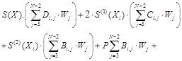
![]() ,
, ![]() (13)
(13)
where![]() ,
,![]() is the functional value at the grid
is the functional value at the grid![]() ,
, ![]() ,
, ![]() and
and ![]() is the weighting coefficient matrix of the second, third and forth order derivatives.
is the weighting coefficient matrix of the second, third and forth order derivatives. ![]() ,
, ![]() are the second and first order derivatives of
are the second and first order derivatives of ![]() at
at![]() . Similarly, the derivatives in the boundary conditions can be discretized by the GDQ method. As a result, the numerical boundary conditions can be written as:
. Similarly, the derivatives in the boundary conditions can be discretized by the GDQ method. As a result, the numerical boundary conditions can be written as:
![]() (14a)
(14a)
![]() (14b)
(14b)
![]() (14c)
(14c)
![]() (14d)
(14d)
where n0, n1 may be taken as either 1 or 2. By choosing the value of n0 and n1, Equation (20) can give the following four sets of boundary conditions,
n0 = 1, n1 = 1 ـــــــــــــــ clamped–clamped supported
n0 = 1, n1 = 2 ـــــــــــــــ clamped–simply supported
n0 = 2, n1 = 1 ــــــــــــــ simply–clamped supported
n0 = 2, n1 = 2 ـــــــــــــــ simply–simply supported
Equations (14a) and (14c) can be easily substituted into the governing equation. This is not the case for Equations (14b) and (14d). However, one can couple these two equations together to give two solutions, ![]() and
and![]() , as
, as
![]() (15a)
(15a)
![]() (15b)
(15b)
where
![]()
![]()
![]()
According to Equations (15), ![]() and
and![]() are expressed in terms of
are expressed in terms of![]() , and can be easily substituted into the governing equation (13). It should be noted that Equation (14) provides four boundary equations. In total we have N unknowns
, and can be easily substituted into the governing equation (13). It should be noted that Equation (14) provides four boundary equations. In total we have N unknowns![]() . In order to close the system, the discretized governing equation (13) has to be applied at
. In order to close the system, the discretized governing equation (13) has to be applied at ![]() mesh points. This can be done by applying Equation (13) at grid points
mesh points. This can be done by applying Equation (13) at grid points![]() Substituting Equations (14a), (14c) and (15) into Equation (13) gives:
Substituting Equations (14a), (14c) and (15) into Equation (13) gives:
![]() ,
, ![]() (16)
(16)
It is noted that Equation (16) has ![]() equations with
equations with ![]() unknowns, which can be written in matrix eigen-value form as;
unknowns, which can be written in matrix eigen-value form as;
![]() (17)
(17)
where ![]()
The Matlab program has been used to solve this eigen-value problem and get the normalized frequencies Ω and the corresponding mode shapes.
4. Results and Discussion
In this section we will analyze the vibration of uniform and non-uniform beams resting on fluid layer under axial force, we will calculating the natural frequencies and corresponding mode shapes of uniform and non-uniform beams under three sets of boundary conditions, that is, simply supported–simply supported (S–S), clamped–clamped supported (C–C) and clamped–simply supported (C–S). By using the differential quadrature method, using the method of directly Substitutes the Boundary Conditions into the Governing Equations is referred to as (SBCGE).
In the present study, the coordinates of the grid points for the beam are chosen according to Chebyshev-Gauss-Lobatto by using N sampling as:
![]()
![]()
Table 1a. First three non-dimensional frequencies of uniform Simply–Simply beam
| Natural Frequency | Ω1 | Ω2 | Ω3 |
| Exact (Belvins [6], Qiang [13]) for uniform beam | 9.8696 | 39.4784 | 88.8264 |
| SBCGM (for uniform beam) | 9.8696 | 39.4784 | 88.8249 |
| SBCGM (for uniform beam resting on fluid, (Kf=1)) | 9.9201 | 39.4911 | 88.8305 |
| SBCGM (for uniform beam resting on fluid under axial force, (Kf=1, P=1)) | 9.4095 | 39.9880 | 88.3292 |
Table 1b. First three non-dimensional frequencies of uniform Clamped–Clamped beam
| Natural Frequency | Ω1 | Ω2 | Ω3 |
| Exact (Belvins [6], Qiang [13]) for uniform beam | 22.3733 | 61.6728 | 120.9034 |
| SBCGM (for uniform beam) | 22.3733 | 61.6728 | 120.9034 |
| SBCGM (for uniform beam resting on fluid, (Kf=1)) | 22.3956 | 61.6809 | 120.9062 |
| SBCGM (for uniform beam resting on fluid under axial force, (Kf =1, P=1)) | 22.1191 | 61.3064 | 120.4965 |
Table 1c. First three non-dimensional frequencies of uniform Clamped–Simply beam
| Natural Frequency | Ω1 | Ω2 | Ω3 |
| Exact (Belvins [6], Qiang [13]) for uniform beam | 15.4182 | 49.9648 | 104.2477 |
| SBCGM (for uniform beam) | 15.4182 | 49.9648 | 104.2471 |
| SBCGM (for uniform beam resting on fluid, (Kf =1)) | 15.4506 | 49.9748 | 104.2519 |
| SBCGM (for uniform beam resting on fluid under axial force, (Kf =1, P=1)) | 15.0731 | 49.5438 | 103.7999 |
Numerical calculations have been done for both a uniform beam ![]() and a non-uniform beam under three sets of boundary conditions, namely simply–simply supported (S–S), clamped–clamped supported (C–C) and clamped–simply supported (C–S). The GDQ results using the present approach for implementation boundary conditions are compared with the well known exact solution (cf. Belvins) [6] and the exact solution (Qiang) [13] for uniform beam. Table 1 lists natural frequencies for the first three modes of a uniform beam resting on fluid layer under axial force. Included in Table 1 are SBCGE results for uniform beam, the SBCGE results for uniform beam resting on fluid layer, the SBCGE results for uniform beam resting on fluid layer under axial force, the exact solution (Qiang) [13] and the exact solutions (cf. Belvins) [6] for uniform beam. The GDQ results are obtained using 15 non-uniformly spaced grid points. It can be observed from Table 1 that, the SBCGE results agree very well with the exact solutions. Also, It can be observed from Table 1 that, the natural frequencies increases when the beam resting on fluid layer while decreases when the beam resting on fluid layer under axial force.
and a non-uniform beam under three sets of boundary conditions, namely simply–simply supported (S–S), clamped–clamped supported (C–C) and clamped–simply supported (C–S). The GDQ results using the present approach for implementation boundary conditions are compared with the well known exact solution (cf. Belvins) [6] and the exact solution (Qiang) [13] for uniform beam. Table 1 lists natural frequencies for the first three modes of a uniform beam resting on fluid layer under axial force. Included in Table 1 are SBCGE results for uniform beam, the SBCGE results for uniform beam resting on fluid layer, the SBCGE results for uniform beam resting on fluid layer under axial force, the exact solution (Qiang) [13] and the exact solutions (cf. Belvins) [6] for uniform beam. The GDQ results are obtained using 15 non-uniformly spaced grid points. It can be observed from Table 1 that, the SBCGE results agree very well with the exact solutions. Also, It can be observed from Table 1 that, the natural frequencies increases when the beam resting on fluid layer while decreases when the beam resting on fluid layer under axial force.
To demonstrate better the accuracy of the solutions, the mode shapes of the first three modes of uniform beam resting on fluid layer under axial force were also obtained for three sets of boundary conditions by using 15 non-uniformly spaced grid points. The mode shapes are presented in Figures 1.
Also, Table 2, 3 lists natural frequencies of the first three modes for a non-uniform beams resting on fluid layer under axial force with different stiffness distributions![]() , the first case
, the first case ![]() ,
, ![]() and the second case
and the second case ![]() ,
, ![]() , respectively. Again, three sets of boundary conditions, (S–S, C–C and C–S), were considered for each beam. Also, the GDQ results are obtained using 15 non-uniformly spaced grid points. The varying cross section stiffness S(X) of the beams can be very easily implemented from equations (22). The computing effort is still small since one has to solve an eigen-value problem of a matrix of dimension 11 × 11 only. Included in Table 2, 3 are GDQ results for non-uniform beam (Du, (1995)) if available, the SBCGE results for non-uniform beam resting on fluid layer and the SBCGE results for non-uniform beam resting on fluid layer under axial force. It can be observed from Table 2, 3 that, the natural frequencies increases when the beam resting on fluid layer while decreases when the beam resting on fluid layer under axial force.
, respectively. Again, three sets of boundary conditions, (S–S, C–C and C–S), were considered for each beam. Also, the GDQ results are obtained using 15 non-uniformly spaced grid points. The varying cross section stiffness S(X) of the beams can be very easily implemented from equations (22). The computing effort is still small since one has to solve an eigen-value problem of a matrix of dimension 11 × 11 only. Included in Table 2, 3 are GDQ results for non-uniform beam (Du, (1995)) if available, the SBCGE results for non-uniform beam resting on fluid layer and the SBCGE results for non-uniform beam resting on fluid layer under axial force. It can be observed from Table 2, 3 that, the natural frequencies increases when the beam resting on fluid layer while decreases when the beam resting on fluid layer under axial force.
From the tables, the convergence of this method is seen to be very good. Accurate results can be achieved by using very few grid points.
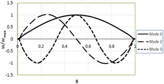
Figure (1a). First three mode shapes of uniform Simply-Simply beam (Kf=1.0, P=1.0).
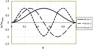
Figure (1b). First three mode shapes of uniform Clamped-Clamped beam (Kf=1.0, P=1.0).
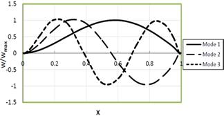
Figure (1c). First three mode shapes of uniform Clamped-Simply beam (Kf=1.0, P=1.0).
To demonstrate better the accuracy of the solutions, the mode shapes of the first three modes of uniform beam resting on fluid layer under axial force were also obtained for three sets of boundary conditions by using 15 non-uniformly spaced grid points. The mode shapes are presented in Figures 2, 3. Figures 2 for the first case ![]() ,
, ![]() , and Figures 3 for the second case
, and Figures 3 for the second case ![]() ,
, ![]() .
.
Table 2a. First three non-dimensional frequencies of non-uniform (S–S) beam (α1 = 0.5, α2 = 1)
| Natural Frequency | Ω1 | Ω2 | Ω3 |
| SBCGM (for non-uniform beam) | 11.0035 | 43.9763 | 98.9180 |
| SBCGM (for non-uniform beam resting on fluid, (Kf=1)) | 11.0489 | 43.9877 | 98.9231 |
| SBCGM (for non-uniform beam resting on fluid under axial force, (Kf=1, P=1)) | 10.5923 | 43.5357 | 98.4720 |
Table 2b. First three non-dimensional frequencies of uniform (C–C) beam (α1 = 0.5, α2 = 1)
| Natural Frequency | Ω1 | Ω2 | Ω3 |
| SBCGM (for non-uniform beam) | 24.8883 | 68.6339 | 134.5731 |
| SBCGM (for non-uniform beam resting on fluid, (Kf=1)) | 24.9084 | 68.6412 | 134.5768 |
| SBCGM (for non-uniform beam resting on fluid under axial force, (Kf=1, P=1)) | 24.6599 | 68.3046 | 98.4720 |
Table 2c. First three non-dimensional frequencies of uniform (C–S) beam (α1 = 0.5, α2 = 1)
| Natural Frequency | Ω1 | Ω2 | Ω3 |
| SBCGM (for non-uniform beam, Du [10])) | 16.9280 | 55.4090 | 115.4800 |
| SBCGM (for non-uniform beam) | 16.9279 | 55.3994 | 115.8263 |
| SBCGM (for non-uniform beam resting on fluid, (Kf=1)) | 16.9574 | 55.4085 | 115.8306 |
| SBCGM (for non-uniform beam resting on fluid under axial force, (Kf=1, P=1)) | 16.6218 | 55.0250 | 115.4272 |
Table 3a. First three non-dimensional frequencies of non-uniform (S–S) beam (α1 = -1, α2 = 1)
| Natural Frequency | Ω1 | Ω2 | Ω3 |
| SBCGM (for non-uniform beam) | 6.3249 | 24.6150 | 53.5371 |
| SBCGM (for non-uniform beam resting on fluid, (Kf =1)) | 6.4035 | 24.6353 | 53.5465 |
| SBCGM (for non-uniform beam resting on fluid under axial force, (Kf =1, P=1)) | 5.5306 | 23.7378 | 52.5812 |
Table 3b. First three non-dimensional frequencies of non-uniform (C–C) beam (α1 = -1, α2 = 1)
| Natural Frequency | Ω1 | Ω2 | Ω3 |
| SBCGM (for non-uniform beam) | 11.9742 | 34.3839 | 68.3635 |
| SBCGM (for non-uniform beam resting on fluid, (Kf=1)) | 12.0159 | 34.3984 | 68.3708 |
| SBCGM (for non-uniform beam resting on fluid under axial force, (Kf=1, P=1)) | 11.4527 | 33.6574 | 67.5535 |
Table 3c. First three non-dimensional frequencies of non-uniform (C–S) beam (α1 = -1, α2 = 1)
| Natural Frequency | Ω1 | Ω2 | Ω3 |
| SBCGM (for non-uniform beam, Du [10])) | 10.7390 | 31.6930 | 65.3110 |
| SBCGM (for non-uniform beam) | 10.3991 | 31.1571 | 63.4720 |
| SBCGM (for non-uniform beam resting on fluid, (Kf=1)) | 10.4471 | 31.1731 | 63.4799 |
| SBCGM (for non-uniform beam resting on fluid under axial force, (Kf=1, P=1)) | 9.7553 | 30.3305 | 62.5810 |
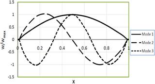
Figure (2a). First three mode shapes of non-uniform Simply-Simply beam (Kf=1.0, P=1.0, α1=0.5, α2=1.0).
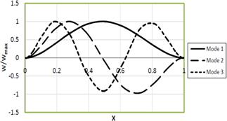
Figure (2b). First three mode shapes of non-uniform Clamped-Clamped beam (Kf=1.0, P=1.0, α1=0.5, α2=1.0).
Figure (2c). First three mode shapes of non-uniform Clamped-Simply beam (Kf=1.0, P=1.0, α1=0.5, α2=1.0).
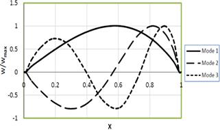
Figure (3a). First three mode shapes of non-uniform Simply-Simply beam (Kf=1.0, P=1.0, α1=-1.0, α2=1.0).
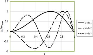
Figure (3b). First three mode shapes of non-uniform Clamped-Clamped beam (Kf=1.0, P=1.0, α1=-1.0, α2=1.0).
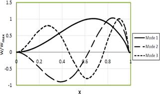
Figure (3c). First three mode shapes of non-uniform Clamped-Simply beam (Kf=1.0, P=1.0, α1=-1.0, α2=1.0).
References
- Bellman, R. E., J. Casti, 1971.Differential quadrature and long-term integration. Journal of Mathematical Analysis and Applications, 34: 235–238.
- Bellman, R. E., B. G. Kashef and J. Casti, 1972. Differential quadrature: A technique for the rapid solution of non-linear partial differential equations. Journal of computational Physics 10: 40–52.
- Bert, C. W., Jang, S. K. and Striz A. G. 1988. Two new methods for analyzing free vibration of structure components. AIAA Journal, 26: 612–618.
- Bert, C., Wang, X. and Striz, A. G. 1993. Differential quadrature for static and free vibration analysis of anisotropic plates. International Journal of Solids Structures 30: 1737–1744.
- Bert, C., Wang, X. and Striz, A. G. 1994. static and free vibrational analysis of beams and plates by differential quadrature method. Acta Mechanica 102: 11–24.
- Blevins, R. D., 1984. Formulas for Natural Frequency and Mode Shapes. Malabur, Florida. Robert E. Krieger.
- Civan, F., and Sliepcevich, C. M., 1984.Differential quadrature for multi-dimensional problems.Journal of Mathematical Analysis Applied 101: 423–443.
- Civan, F., and Sliepcevich, C. M., 1983. Application of differential quadrature to transport processes. Journal of Mathematical Analysis Applied 93: 711–724.
- Du, H., Lim, M. K. and Lin, R. M., 1994. Application of Generalized Differential Quadrature to Structural problems. Journal of Sound and Vibrations 181: 279–293.
- Du, H., Lim, M. K. and Lin, R. M., 1995. Application of Generalized Differential Quadrature to Vibration Analysis. Journal of Sound and Vibrations 181: 279–293.
- Jang, S. K., Bert, C. W. and Striz A. G., 1989. Application of differential quadrature to static analysis of Structural components. International Journal of Numerical Methods in Engineering 28: 561–577.
- Quan, J. R., and Chang C. T., 1989. New insights in solving distributed system equations by the quadrature method-I, analysis. Journal of Computers and Chemical Engineering 13: 779–788.
- Qiang Guo and Zhong, H., 2004. Non-linear Vibration Analysis of Beams by a Spline-based differential quadrature. Journal of Sound and Vibration 269: 405–432.
- Shu, C. and Richards, B. E., 1990. High resolution of natural convection in a square cavity by generalized differential quadrature. Proceedings of 3rd International Conference on Advanced in numerical Methods in Engineering: Theory and Applications, Swansea, U.K 2: 978–985.
- Shu, C., 1991. Generalized differential-integral quadrature and application to the simulation of incompressible viscous flows including parallel computation. PhD thesis, University of Glasgow.
- Shu, C., 2000. Differential Quadrature and its Application in Engineering. Springer, Berlin.
- Wen, D., and Yu, Y., 1993a. Calculation and analysis of weighting coefficient matrices in differential quadrature method. Computational Engineering. Elsevier Oxford 157–162.
- Wen, D., and Yu, Y., 1993b: "Differential quadrature method for high order boundary value problems." In computational Engineering (Edited by Kwak, B. M. and Tanaka, M.): pp. 163–168. Elsevier Oxford.


