
International Journal of Mathematics and Computational Science, Vol. 1, No. 3, June 2015 Publish Date: May 20, 2015 Pages: 141-146
Frequency Analysis of Annual Maximum Flood Discharge Using Method of Moments and Maximum Likelihood Method of Gamma and Extreme Value Family of Probability Distributions
N. Vivekanandan*
Central Water and Power Research Station, Pune, India
Abstract
Estimation of Maximum Flood Discharge (MFD) for a given return period is important for planning, design and management of hydraulic structures for the project. This can be achieved through Flood Frequency Analysis (FFA) by fitting of probability distributions to the recorded Annual Maximum Discharge (AMD) data. In this paper, Gamma and Extreme Value family of probability distributions are adopted in FFA. Method of Moments and Maximum Likelihood Method are used for determination of parameters of six probability distributions. Goodness-of-Fit tests such as Chi-square and Kolmogorov-Smirnov are applied for checking the adequacy of fitting of probability distributions to the recorded AMD data. Diagnostic test of D-index is used for the selection of a suitable distribution for estimation of MFD. The study showed that the exponential distribution (using MLM) is found to be better suited amongst six distributions adopted in estimation of MFD at Dedtalai and gamma distribution (using MLM) for Ghala.
Keywords
Chi-square, D-index, Kolmogorov-Smirnov, Maximum Flood, Probability Distribution
Received: April 3, 2015 / Accepted: April 22, 2015 / Published online: May 19, 2015
@ 2015 The Authors. Published by American Institute of Science. This Open Access article is under the CC BY-NC license. http://creativecommons.org/licenses/by-nc/4.0/
Contents
1. Introduction 2. Methodology 2.1. Theoretical Descriptions of MoM 2.2. Theoretical Descriptions of MLM 2.3. Goodness-of-Fit Tests 2.4. Diagnostic Test 3. Application 4. Results and Discussions 4.1. Estimation of MFD by Six Probability Distributions 4.2. Analysis Based on GoF Tests 4.3. Analysis Based on Diagnostic Test 5. Conclusions Acknowledgements
1. Introduction
For proper planning and design of hydraulic structures like dams, spillways, culverts, etc., a reliable estimation of Maximum Flood Discharge (MFD) for a given return period at the site of interest is necessary. Since the hydrologic phenomena governing the MFD are highly stochastic in nature, the MFD can be effectively determined by fitting of probability distributions to the series of recorded Annual Maximum Discharge (AMD) data through Flood Frequency Analysis (FFA).
A number of probability distributions viz., Exponential (EXP), Gamma (GAM), Generalized Extreme Value (GEV), Generalized Pareto (GPA), Extreme Value Type-1 (EV1) and Pearson Type-3 (PR3) are commonly used in FFA (Khosravi et al., 2012). According to the theory of probability distributions, EXP, GAM and PR3 are called as gamma family of distributions whereas EV1, GEV and GPA are called as extreme value family of distributions. Generally, Method of Moments (MoM) is used for determination of parameters of the probability distribution because of (i) MoM is often simple to derive; (ii) MoM is consistent estimators for continuous type of probability distributions; and (iii) MoM provide initial values in search for maximum likelihood estimates (Hosking and Wallis, 1993). In view of the above, in the present study, MoM and Maximum Likelihood Method (MLM) are used for determination of parameters of probability distributions.
In the recent past, number of studies has been carried out by researchers adopting GAM and Extreme Value family of probability distributions for FFA. Kumar et al. (2003) carried out regional FFA adopting twelve frequency distributions and found that the GEV is better suited distribution for eight gauging sites of middle Ganga plains. Lee (2005) expressed that the PR3 distribution is better suited amongst five distributions studied for analyzing the rainfall distribution characteristics of Chia-Nan plain area. Bhakar et al. (2006) studied the frequency analysis of consecutive day’s maximum rainfall at Banswara, Rajasthan, India. Study by Saf (2009) revealed that the PR3 distribution is better suited for modelling of extreme values in Antalya and Lower-West Mediterranean sub-regions whereas the Generalized Logistic distribution for the Upper-West Mediterranean sub-region.
Mujere (2011) applied EV1 distribution for modelling flood data for the Nyanyadzi River, Zimbabwe. Baratti et al. (2012) carried out FFA on seasonal and annual time scales for the Blue Nile River adopting EV1 distribution. Esteves (2013) applied extreme value distributions to estimate the extreme precipitation depths at different rain-gauge stations in southeast United Kingdom. Izinyon and Ajumuka (2013) carried out FFA for three tributaries of upper Benue river basin, Nigeria adopting Log-normal, EV1 and Log Pearson Type-3 (LP3) distributions. Das and Qureshi (2014) evaluated the probability distributions of GEV, LP3 and LN2 adopted in FFA through D-index and found that the LP3 is better suited distribution for estimation of MFD for Jiya Dhol river basin. But, there is no general agreement in applying a particular distribution for a region or country. This can be answered by formal statistical procedures involving Goodness-of-Fit (GoF) and diagnostic tests; and the results are quantifiable and reliable (Zhang, 2002). For quantitative assessment on MFD within in the recorded range, Chi-square (c2) and Kolmogorov-Smirnov (KS) tests are applied. A diagnostic test of D-index is used for the selection of suitable probability distribution for estimation of MFD (USWRC, 1981). Qualitative assessment is made from the plots of the recorded and estimated MFD. In the present study, comparison of Gamma and Extreme Value family of probability distributions is made which also illustrates the applicability of GoF and diagnostic tests procedures in identifying the best suitable distribution for estimation of MFD for river Tapi at Dedtalai and Ghala gauging sites.
2. Methodology
The study is to assess the probability distribution for FFA. Thus, it is required to process and validate the data for application such as (i) select the Probability Density Functions (PDFs) for FFA (say, EXP, EV1,GAM, GEV, GPA and PR3); (ii) determine the parameters of distributions using MoM and MLM; (iii) select quantitative GoF and diagnostic tests and (iv) conduct FFA and analyse the results obtained thereof. Table 1 gives the PDFs with the corresponding flood quantile estimators of six probability distributions used in FFA.
Table 1. PDFs with flood quantile estimators (![]() )
)
| Distribution | ||
| EXP |
|
|
| GAM |
|
|
| PR3 |
|
|
| EV1 |
|
|
| GEV |
|
|
| GPA |
|
|
where, F(Q) (or F) is the Cumulative Distribution Function (CDF) of Q and KP is the frequency factor corresponding to CS. For GAM distribution, CS is computed from![]() . Similarly, for PR3 distribution, CS is computed from the series of AMD.
. Similarly, for PR3 distribution, CS is computed from the series of AMD. ![]() ,
,![]() and
and![]() are the location, scale and shape parameters respectively.
are the location, scale and shape parameters respectively. ![]() is the estimated MFD by probability distribution corresponding to return period T.
is the estimated MFD by probability distribution corresponding to return period T.
2.1. Theoretical Descriptions of MoM
MoM is a technique for constructing estimators of the parameters that is based on matching the sample moments with the corresponding distribution moments (Haktanir and Horlacher, 1993; Ghorbani et al., 2010). The rth central moment (![]() ) about the mean (
) about the mean (![]() ) of a random variable Q is defined by:
) of a random variable Q is defined by:
![]() , if Q is continuous variable(1)
, if Q is continuous variable(1)
where, f(Q) is a PDF of a random variable Q. The second moment (![]() ) about
) about ![]() is called as variance. Similarly, third and fourth moments (
is called as variance. Similarly, third and fourth moments (![]() and
and ![]() ) about
) about ![]() are used to define skewness (CS) and kurtosis (CK), which are as follows:
are used to define skewness (CS) and kurtosis (CK), which are as follows:
![]() and
and ![]() (2)
(2)
2.2. Theoretical Descriptions of MLM
The probability of occurrence of an observed sample series of a random variable can be calculated by multiplying the PDFs of every single observed data of that series with each other on the assumption that the events of the random variable are independent, which results in the Likelihood Function (LF). The parameter values that make the LF maximum will be the most suitable ones for that sample series because it actually happened among so many other possible sample series of the population. The maximum values of the LF and the logarithm of the LF always coincide with the same magnitudes of the distribution parameters. Therefore, it is analytically more convenient to take the derivative of the logarithm of the LF, which consists of summations of logarithms of the PDF, namely, LLF. For example, LF and LLF for 2-parameter and 3-parameter probability distributions are as given below.
LF =![]() and LLF=
and LLF=![]() (3)
(3)
LF ![]() =and LLF=
=and LLF=![]() (4)
(4)
A system of non-linear equations can be obtained from the analytical expressions of the partial derivatives of each parameter through LLF. The roots that make all these equations zero simultaneously are the magnitudes of the parameters estimated by MLM (Seckin et al., 2010). The procedures involved in determination of parameters of probability distributions (using MoM and MLM) are briefly described in the text book of ‘Flood Frequency Analysis’ by Rao and Hamed (2000).
2.3. Goodness-of-Fit Tests
GoF tests are essential for checking the adequacy of probability distributions to the recorded series of AMD in the estimation of MFD. Out of a number GoF tests available, the widely accepted GoF tests are c2 and KS, which are used in the study. The theoretical descriptions of GoF tests statistic are as follows:
c2 Statistic:
![]() (5)
(5)
where, ![]() is the observed frequency value of jthclass,
is the observed frequency value of jthclass, ![]() is the expected frequency value of jthclass and NC is the number of frequency classes. The rejection region of c2 statistic at the desired significance level (h) is given by
is the expected frequency value of jthclass and NC is the number of frequency classes. The rejection region of c2 statistic at the desired significance level (h) is given by![]() . Here, m denotes the number of parameters of the distribution and
. Here, m denotes the number of parameters of the distribution and ![]() is the computed value of c2 statistic by PDF.
is the computed value of c2 statistic by PDF.
KS Statistic:
![]() (6)
(6)
where, ![]() is the empirical CDF of
is the empirical CDF of ![]() and
and![]() is the computed CDF of
is the computed CDF of ![]() (Zhang, 2002).
(Zhang, 2002).
Test criteria: If the computed values of GoF tests statistic given by the distribution are lesser than that of the theoretical values at the desired significance level, then the distribution is considered to be acceptable for estimation of MFD.
2.4. Diagnostic Test
The selection of a suitable probability distribution for estimation of MFD is carried out through D-index, which is defined as:
D-index =![]() (7)
(7)
where, ![]() is the average (or mean) of the recorded AMD,
is the average (or mean) of the recorded AMD,![]() ’s (i=1 to 6) are the first six highest sample values in the series and
’s (i=1 to 6) are the first six highest sample values in the series and ![]() is the estimated value by PDF. The distribution having the least D-index is identified as better suited distribution in comparison with the other distributions for estimation of MFD (Vivekanandan, 2014).
is the estimated value by PDF. The distribution having the least D-index is identified as better suited distribution in comparison with the other distributions for estimation of MFD (Vivekanandan, 2014).
3. Application
In this paper, a study was carried out to estimate the MFD adopting six probability distributions on river Tapi at Dedtalai and Ghala gauging sites. Based on the water year (June-May), stream flow data related to the period 1977-78 to 2004-05 for Dedtalai and 1978-79 to 2004-05 for Ghala is used. The series of AMD is derived from the daily stream flow data and used in FFA. Table 2 gives the summary statistics of AMD.
Table 2. Summary statistics of AMD
| Gauging site | Statistical parameters (SD: Standard Deviation) | |||
| Mean (m3/s) | SD (m3/s) | Skewness | Kurtosis | |
| Dedtalai | 3441.9 | 3533.3 | 2.643 | 9.323 |
| Ghala | 3563.9 | 4901.4 | 1.801 | 1.994 |
4. Results and Discussions
Statistical software, namely VTFIT, is used in FFA. This software gives the parameters of the six probability distributions (using MoM and MLM), MFD estimates for different return periods, GoF and diagnostic tests results.
4.1. Estimation of MFD by Six Probability Distributions
The parameters of six probability distributions are determined by MoM and MLM; and further used for estimation of MFD. Tables 3 and 4 give the estimates of MFD for different return periods for river Tapi at Dedtalai and Ghala sites. The MFD estimates are used to develop the flood frequency curves and presented in Figures 1 and 2.
4.2. Analysis Based on GoF Tests
In the present study, the degree of freedom (NC-m-1) was considered as one for 3-parameter distributions (PR3, GEV and GPA) and two for 2-parameter distributions (EXP, GAM and EV1) while computing the c2 statistic values for Dedtalai and Ghala. GoF tests statistic is computed using Eqs. (5) and (6); and the results are presented in Table 5.
From Table 5, it may be noted that the computed values of c2 statistic for EXP, GAM and EV1 distributions (using MoM and MLM) are lesser than the theoretical values at 5% significance level and thus these three distributions are acceptable at 5% significance level for Dedtalai. On the other hand, the computed values of c2 statistic by the distributions are greater than the theoretical values at 5% significance level and all six distributions are not acceptable at 5% significance level for Ghala when MoM and MLM is applied for determination of parameters of the distributions.
For Dedtalai, it may be noted that the computed values of KS statistic by six probability distributions (using MoM and MLM) are lesser than the theoretical value at 5% significance level and therefore all six distributions are acceptable for estimation of MFD. Also, from Table 5, it may be noted that the computed values of KS statistic by GAM, PR3 and GEV distributions (using MoM and MLM) are lesser than the theoretical value at 5% significance level and at this level these three distributions are acceptable for estimation of MFD at Ghala.
4.3. Analysis Based on Diagnostic Test
For the selection of the best suitable distribution for estimation of MFD, the D-index values of six probability distributions are computed from Eq. (7) and given in Table 6.
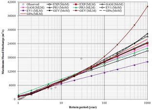
Figure 1. Plots of recorded and estimated MFD by six probability distributions (using MoM and MLM) for river Tapi at Dedtalai
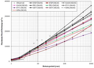
Figure 2. Plots of recorded and estimated MFD by six probability distributions (using MoM and MLM) for river Tapi at Ghala
Table 3. MFD estimates for different return periods for river Tapi at Dedtalai
| Return period (year) | Estimated MFD (m3/s) | |||||||||||
| MoM | MLM | |||||||||||
| EXP | GAM | PR3 | EV1 | GEV | GPA | EXP | GAM | PR3 | EV1 | GEV | GPA | |
| 2 | 2358 | 2335 | 2128 | 2861 | 2630 | 2326 | 2372 | 2426 | 3886 | 2870 | 2484 | 2625 |
| 5 | 5595 | 5562 | 5175 | 5985 | 5422 | 5308 | 5567 | 5520 | 6666 | 5182 | 5064 | 5633 |
| 10 | 8044 | 8028 | 7795 | 8053 | 7564 | 7720 | 7985 | 7842 | 8719 | 6712 | 7304 | 7999 |
| 20 | 10493 | 10504 | 10552 | 10037 | 9870 | 10277 | 10402 | 10157 | 10750 | 8180 | 9963 | 10447 |
| 50 | 13731 | 13787 | 14327 | 12605 | 13270 | 13891 | 13598 | 13209 | 13414 | 10080 | 14342 | 13813 |
| 100 | 16180 | 16276 | 17248 | 14529 | 16164 | 16815 | 16015 | 15514 | 15420 | 11504 | 18493 | 16461 |
| 200 | 18629 | 18768 | 20211 | 16446 | 19381 | 19914 | 18433 | 17817 | 17419 | 12923 | 23557 | 19201 |
| 500 | 21867 | 22065 | 24174 | 18976 | 24200 | 24295 | 21628 | 20858 | 20054 | 14794 | 32009 | 22968 |
| 1000 | 24316 | 24562 | 27200 | 20887 | 28332 | 27839 | 24046 | 23157 | 22043 | 16209 | 40070 | 25932 |
Table 4. MFD estimates for different return periods for river Tapi at Ghala
| Return period (year) | Estimated MFD (m3/s) | |||||||||||
| MoM | MLM | |||||||||||
| EXP | GAM | PR3 | EV1 | GEV | GPA | EXP | GAM | PR3 | EV1 | GEV | GPA | |
| 2 | 2060 | 1701 | 2184 | 2758 | 2558 | 2089 | 2265 | 2241 | 2541 | 2614 | 1944 | 2014 |
| 5 | 6551 | 5865 | 6717 | 7092 | 6682 | 6711 | 6144 | 5822 | 6086 | 5445 | 4188 | 5329 |
| 10 | 9948 | 9530 | 10022 | 9961 | 9651 | 10108 | 9077 | 8652 | 8623 | 7319 | 5943 | 7801 |
| 20 | 13346 | 13420 | 13275 | 12713 | 12691 | 13420 | 12011 | 11533 | 11099 | 9116 | 7861 | 10241 |
| 50 | 17837 | 18777 | 17527 | 16275 | 16927 | 17673 | 15890 | 15391 | 14315 | 11443 | 10739 | 13421 |
| 100 | 21234 | 22938 | 20718 | 18944 | 20339 | 20797 | 18824 | 18334 | 16718 | 13187 | 13230 | 15792 |
| 200 | 24632 | 27166 | 23893 | 21604 | 23956 | 23844 | 21757 | 21293 | 19103 | 14924 | 16040 | 18133 |
| 500 | 29123 | 32833 | 28072 | 25112 | 29083 | 27757 | 25636 | 25222 | 22234 | 17216 | 20322 | 21183 |
| 1000 | 32520 | 37165 | 31222 | 27764 | 33246 | 30631 | 28570 | 28205 | 24590 | 18949 | 24054 | 23457 |
Table 5. Computed and theoretical values of GoF tests statistic
| Distribution | Computed values of GoF tests statistic | Theoretical values of GoF tests statistic | ||||||||
| Dedtalai | Ghala | |||||||||
| c2 | KS | c2 | KS | |||||||
| MoM | MLM | MoM | MLM | MoM | MLM | MoM | MLM | c2 | KS | |
| EXP | 4.143 | 4.143 | 0.119 | 0.137 | 17.259 | 9.852 | 0.255 | 0.317 | 5.990 | 0.250 (for Dedtalai) |
| GAM | 4.143 | 4.143 | 0.122 | 0.148 | 13.556 | 22.444 | 0.194 | 0.249 | 5.990 | |
| PR3 | 9.143 | 5.929 | 0.152 | 0.192 | 17.259 | 7.630 | 0.252 | 0.188 | 3.840 | |
| EV1 | 3.786 | 2.714 | 0.126 | 0.154 | 38.370 | 38.370 | 0.258 | 0.285 | 5.990 | 0.254 (for Ghala) |
| GEV | 4.500 | 4.452 | 0.083 | 0.090 | 39.111 | 38.752 | 0.250 | 0.183 | 3.840 | |
| GPA | 6.286 | 4.857 | 0.120 | 0.107 | 17.259 | 10.593 | 0.263 | 0.275 | 3.840 | |
Table 6. D-index values of probability distributions
| Gauging site | Indices of D-index | |||||||||||
| MoM | MLM | |||||||||||
| EXP | GAM | PR3 | EV1 | GEV | GPA | EXP | GAM | PR3 | EV1 | GEV | GPA | |
| Dedtalai | 3.346 | 3.307 | 2.881 | 3.901 | 3.336 | 3.097 | 3.352 | 3.397 | 4.347 | 3.796 | 2.865 | 3.332 |
| Ghala | 4.005 | 4.106 | 4.077 | 4.547 | 4.520 | 3.965 | 5.057 | 5.556 | 5.777 | 7.547 | 9.691 | 6.798 |
By using the diagnostic test results presented in Table 6, the following observations are drawn from the study.
i) The indices of D-index of 2.881 (using PR3) for Dedtalai and 3.965 (using GPA) for Ghala are comparatively minimum when MoM is applied for determination of parameters of the distributions.
ii) Likewise, the indices of D-index of 2.865 (using GEV) for Dedtalai and 5.057 (using EXP) for Ghala are comparatively minimum when MLM is applied for determination of parameters of the distributions.
iii) c2 test results don’t support the use of PR3, GEV and GPA distributions (using MoM and MLM) for estimation of MFD at Dedtalai.
iv) Both c2 and KS tests result don’t support the use of EXP, EV1 and GPA distributions (using MoM and MLM) for estimation of MFD at Ghala.
v) Based on the eliminations of the probability distributions have minimum D-index through GoF (c2 and KS) tests results, it may be noted that:
a) D-index value of 3.307 computed by GAM (using MoM) is the next minimum when compared to the corresponding values of EXP and EV1 for Dedtalai.
b) For Ghala, it may be noted that the D-index value of 4.077 computed by PR3 distribution (using MoM) is the next minimum when compared to the corresponding values of GAM and GEV.
vi) From the research studies, it is observed that the estimated parameters of distributions fitted by MoM are often less accurate than those obtained by MLM. So, the selection of a suitable probability distribution is made through quantitative (using D-index) and qualitative (using probability plots) assessment.
a) The D-index values of 3.352 (for Dedtalai) and 5.556 (for Ghala) computed by EXP and GAM distributions (using MLM) are minimum when compared to the corresponding values of other probability distributions, which are supported by GoF tests.
b) By considering the trend lines of the fitted curves using estimated MFD values, the study identifies the EXP distribution (using MLM) is found to be a good choice for estimation of MFD for Dedtalai whereas GAM distribution (using MLM) for Ghala.
5. Conclusions
The paper describes briefly the study carried out for estimation of MFD by adopting FFA (using VTFIT software) for determination of parameters of six probability distributions (using MoM and MLM) for Dedtalai and Ghala. The following conclusions are drawn from the study:
i) The study presents the selection of suitable distribution evaluated by GoF (using c2 and KS) and diagnostic (using D-index) tests.
ii) The c2 test results showed that the EXP, EV1 and GAM distributions (using MoM and MLM) are acceptable for estimation of MFD at Dedtalai.
iii) The c2 test results showed that the EXP, EV1, GAM, GEV, GPA and PR3 distributions are not acceptable for estimation of MFD at Ghala when MoM and MLM is applied for determination of parameters of distributions.
iv) The KStest results indicated that these six probability distributions are acceptable for estimation of MFD at Dedtalai whereas GAM, GEV and PR3 distributions are acceptable for Ghala when MoM and MLM is applied for determination of parameters of distributions.
v) By considering the trend lines of the fitted curves using estimated MFD values, the study presented that the EXP distribution (using MLM) is better suited amongst six distributions adopted for estimation of MFD for Dedtalai whereas GAM distribution (using MLM) for Ghala.
vi) The study suggested that the MFD values computed by EXP (for Dedtalai) and GAM (for Ghala) distributions (using MLM) could be considered as the design parameter for planning and design of hydraulic structures in the vicinity of the gauging sites.
Acknowledgements
The author is grateful to Shri S. Govindan, Director, Central Water and Power Research Station, Pune, for encouragement given for conducting the studies and also accordingly permission to publish this paper. The author is thankful to the Executive Engineer (Tapi Division), Central Water Commission for providing stream flow data used in the study.
References
- Baratti, E., Montanari, A., Castellarin, A., Salinas, J.L., Viglione, A. and Bezzi, A. (2012); Estimating the flood frequency distribution at seasonal and annual time scales,Hydrology and Earth System Sciences,Vol. 16, No. 12, pp. 4651–4660.
- Bhakar, S.R., Bansal, A.K., Chhajed, N. and Purohit R.C. (2006); Frequency analysis of consecutive days maximum rainfall at Banswara, Rajasthan, India. ARPN Journal of Engineering and Applied Sciences, Vol. 1, No. 3, pp. 64-67.
- Das, L.M. andQureshi, Z.H. (2014);Flood frequency analysis for Jiya Dholriver of Brahmaputravalley,Journal of Sciences: Basic and Applied Research,Vol.14, No.2, pp.14-24.
- Esteves, L.S. (2013); Consequences to flood management of using different probability distributions to estimate extreme rainfall, Journal of Environmental Management, Vol. 115, No. 1, pp. 98-105.
- Ghorbani, A.M., Ruskeep, A.H., Singh, V.P. and Sivakumar, B. (2010); Flood Frequency analysis using mathematica, Turkish Journal of Engineering and Environmental Sciences, Vol. 34, No. 3, pp. 171-188.
- Haktanir, T. and Horlacher, H.B. (1993); Evaluation of various distributions for flood frequency analysis, Hydrological Sciences Journal, Vol. 38, No. 1, pp. 15-32.
- Hosking, J.R.M. and Wallis, J.R. (1993); Some statistics useful in regional frequency analysis, Water Resources Research, Vol. 29, No. 2, pp. 271-281.
- Izinyon, O.C. and Ajumuka, H.N. (2013); Probability distribution models for flood prediction in Upper Benue River Basin, Journal of Civil and Environmental Research, Vo1. 3, No. 2, pp. 62-74.
- Kumar, R., Chatterjee, C., Kumar, S., Lohani, A.K. and Singh, R.D. (2003); Development of regional flood frequency relationships using L-moments for Middle Ganga Plains Subzone 1(f) of India, Water Resources Management, Vol. 17, No. 4, pp. 243–257.
- Khosravi, Gh., Magidi, A. and Nohegar, A. (2012); Determination of suitable probability distribution for annual and peak discharge estimations (Case Study: Minab River-Barantin Gage, Iran). Journal of Probability and Statistics, Vo1. 1, No. 5, pp. 160-163.
- Lee, C. (2005); Application of rainfall frequency analysis on studying rainfall distribution characteristics of Chia-Nan plain area in Southern Taiwan, Journal of Crop, Environment & Bioinformatics, Vol. 2, No. 1, pp. 31-38.
- Mujere, N. (2011); Flood frequency analysis using the Gumbel distribution, Journal of Computer Science and Engineering, Vol. 3, No. 7, pp. 2774-2778.
- Seckin, N., Yurtal, R., Haktanir, T. and Dogan A. (2010);Comparison of probability weighted moments and maximum likelihood methods used in flood frequency analysis for Ceyhan river basin, Arabian Journal for Science and Engineering, Vol. 35, No. 1B , pp. 49-69.
- Rao, A.R. and Hamed, K.H. (2000); Flood frequency analysis, CRC Publications, New York.
- Saf, B. (2009); Regional flood frequency analysis using L-moments for the West Mediterranean Region of Turkey, Water Resources Management, Vol. 23, No. 3, pp. 531-551.
- United States Water Resources Council (1981); Guidelines for determiningfloodflow frequency, Bulletin No. 17B.
- Vivekanandan N. (2014); Frequency analysis of annual 1-day maximum rainfall using extreme value distributions,Fidelity Journals of Physical Sciences Vol. 1, No. 1pp. 1-4.
- Zhang, J. (2002); Powerful goodness-of-fit tests based on the likelihood ratio, Journal of Royal Statistical Society Series B, Vol. 64, pp. 281-294.


