
International Journal of Mathematics and Computational Science, Vol. 1, No. 3, June 2015 Publish Date: May 20, 2015 Pages: 132-140
Numerical Analysis of the Existence and Stability of Spherical Crystals Growing in a Supersaturated Solution
Mohammad Shafique*
Department of Mathematics, Gomal University, Dera Ismail Khan, Pakistan
Abstract
The growth of a spherical amorphous crystal in supersaturated melt is analyzed numerically. The model problem is written in a scaled form which is suitable for numerical solution. Critical radii for the onset of instability to Yl, m bumps are obtained through simulation. These numerical results agree with those obtained previously for limiting values (very small and very large) of the super saturation. Moreover they show that the usual sequence of instabilities (Yl, m followed by Yl+1, m bumps) predicted by the classic Mullins and Sekerka model (valid only for small super saturation) breaks down for large super saturation.
Keywords
Numerical Analysis, Spherical Crystal, Supersaturated Solution
Received: April 1, 2015 / Accepted: April 18, 2015 / Published online: May 19, 2015
@ 2015 The Authors. Published by American Institute of Science. This Open Access article is under the CC BY-NC license. http://creativecommons.org/licenses/by-nc/4.0/
1. Introduction
The shape stability of a spherical particle growing in a diffusion field (for example, growth form supersaturated solution) has been studied theoretically by Chadam et al. [1]. There the authors consider the following mathematical model, which is similar to the classic Mullins and Sekerka model [2,3], but do not impose the quasi-steady-state assumption and replace the diffusion equation by Laplace’s equation. In particular, if c is the concentration of the solute and the solid-solute interface is![]() , then the problem is to find these two quantities subject to:
, then the problem is to find these two quantities subject to:
![]() (1a)
(1a)
![]() (1b)
(1b)
![]() (1c)
(1c)
![]() (1d)
(1d)
![]() . (1e)
. (1e)
For given initial functions![]() . Here, ρ is the density of the solid
. Here, ρ is the density of the solid ![]() is the equilibrium concentration on a planner interface and
is the equilibrium concentration on a planner interface and ![]() is the ambient concentration far from the solid. Also, n is the normal to
is the ambient concentration far from the solid. Also, n is the normal to ![]() and
and ![]() is the normal velocity of the interface. The function
is the normal velocity of the interface. The function ![]() is the mean curvature of the surface
is the mean curvature of the surface ![]() is a measure of the interfacial energy. Thus, in [1], as in the Mullins and Sekerka model, the interaction at the interface is so rapid that it is maintained at equilibrium as given by the Gibbs-Thompson relation (1c).
is a measure of the interfacial energy. Thus, in [1], as in the Mullins and Sekerka model, the interaction at the interface is so rapid that it is maintained at equilibrium as given by the Gibbs-Thompson relation (1c).
The problem (1) is a generalization of the classical one-phase Stefan problem [8,18,20] in that it includes the nonlinear function ![]() in (1b) and
in (1b) and ![]() in (1c) is not constant (which would result from assuming
in (1c) is not constant (which would result from assuming![]() ). Here, as [1], the growing solutions of problem (1) are studied rather than the shrinking ones associated with melting problems.
). Here, as [1], the growing solutions of problem (1) are studied rather than the shrinking ones associated with melting problems.
In [1], the spherical version of the set of equations (1) has been studied along the same lines as in [5,6]. In particular, the existence and uniqueness results for radically symmetric growth of the spherical crystal are obtained, when the ratio ![]() (a measure of super saturation) satisfies
(a measure of super saturation) satisfies ![]() Then the shape stability of the spherical solution to be spherical harmonics (
Then the shape stability of the spherical solution to be spherical harmonics (![]() -modes, for
-modes, for ![]() ) is also examined theoretically by showing that the
) is also examined theoretically by showing that the ![]() similarity solution is marginally stable among all spherical solutions with a given value of S. They have shown that, if
similarity solution is marginally stable among all spherical solutions with a given value of S. They have shown that, if ![]() (i.e., exclusion of surface tension), the spherical harmonics are unstable. Also, they have obtained the quasi-steady-state growth rate
(i.e., exclusion of surface tension), the spherical harmonics are unstable. Also, they have obtained the quasi-steady-state growth rate ![]() for the
for the ![]() -modes. But, this growth rate reduces, if
-modes. But, this growth rate reduces, if ![]() (i.e., inclusion of surface tension), and indeed stability some
(i.e., inclusion of surface tension), and indeed stability some ![]() -modes when the radius is sufficiently small. However, all spherical harmonics grow again when the radius is sufficiently large.
-modes when the radius is sufficiently small. However, all spherical harmonics grow again when the radius is sufficiently large.
Further, they have compared the theoretical results of the radius, at which ![]() -modes stops decaying and starts growing, in terms of the critical radius with the results of Mullins-Sekerka [2,3]. In particular, it has been established that the critical radius at which the crystal becomes unstable is larger for small super saturation and smaller for large super saturation.
-modes stops decaying and starts growing, in terms of the critical radius with the results of Mullins-Sekerka [2,3]. In particular, it has been established that the critical radius at which the crystal becomes unstable is larger for small super saturation and smaller for large super saturation.
We continue to analyze the problem (1) numerically, and then compare our numerical results with the theoretical results of Chadam et al. [1], and with the quasi-steady-state analysis of Mullins and Sekerka [2,3]. In section 2, the spherical symmetric versions of equations (1) are solved numerically and the explicit form of the concentration profile is obtained. In section 3, we derive the formulae necessary to study numerically the shape stability of the spherical solutions to the spherical harmonics (![]() -modes, for
-modes, for![]() ). The numerical methods used in solving the above problem are presented in section 4 while in section 5 the numerical results and the graphical representation of the critical radius for the stability of the solutions are discussed in detail. Section 6, contains the conclusions.
). The numerical methods used in solving the above problem are presented in section 4 while in section 5 the numerical results and the graphical representation of the critical radius for the stability of the solutions are discussed in detail. Section 6, contains the conclusions.
2. Spherical Solutions
For numerical purpose we begin by non-dimensionalizing the equations in order to reduce the number of unknown parameters. Using a new parameter ϴ defined by
![]() , (2)
, (2)
the equations (1) (with D=1) change to
![]() (3a)
(3a)
 (3b)
(3b)
 (3c)
(3c)
![]() (3d)
(3d)
![]() (3e)
(3e)
Where ![]() and
and ![]() is the critical nucleation radius.
is the critical nucleation radius.
Then, scaling with ![]() and
and![]() , we have, with
, we have, with ![]()
![]() (4a)
(4a)
![]() (4b)
(4b)
![]() (4c)
(4c)
![]() (4d)
(4d)
![]() (4e)
(4e)
These are the scaled versions of the equations, involving the single parameter S, which will be useful for numerical study.
Now, the spherical version of the above set of equations with ![]() is
is
![]() (5a)
(5a)
![]() (5b)
(5b)
![]() (5c)
(5c)
![]() (5d)
(5d)
![]() (5e)
(5e)
We note that a similarity solution in the variable ![]() can be computed explicitly using standard methods [4,7,8,17]. Denoting this special solution as,
can be computed explicitly using standard methods [4,7,8,17]. Denoting this special solution as,
![]() (6)
(6)
![]() (7)
(7)
Where![]() and
and![]() are the linearly independent solutions of
are the linearly independent solutions of
![]()
Then as in [1],
![]() (8a)
(8a)
![]() (8b)
(8b)
![]() (8c)
(8c)
![]() (8d)
(8d)
Now, to compute the constants A, B, C, D and β in (7), we use the interface and asymptotic conditions (5b-d). We write (7), using the above equations as:
 (9)
(9)
The boundary conditions (5b) with![]() ,
,
![]() (10a)
(10a)
Also (9) with ![]() becomes
becomes
 (10b)
(10b)
From (10a) and (10b), we have
![]() (11a)
(11a)
![]() (11b)
(11b)
Where![]()
![]()
![]() and
and ![]() .
.
The boundary conditions (5c) with ![]() is
is
![]() (12a)
(12a)
Also using (11a, b) and taking ![]() (9) gives
(9) gives
![]() (12b)
(12b)
Comparing (12a) and (12b), we have
![]() (13a)
(13a)
![]() . (13b)
. (13b)
Now, the system of equations (12a, b) and (13a, b) can be solved by using Cramer’s rule calculating the denominators or the Wronskian directly we get
![]() (14a)
(14a)
![]() (14b)
(14b)
![]() (14c)
(14c)
![]() (14d)
(14d)
Note that, in (9)![]() ,
, ![]() and
and![]() , so that the only contribution to
, so that the only contribution to ![]() is form
is form
 (15)
(15)
But ![]() in (5d), then in (15)
in (5d), then in (15) ![]() . This implies B=0 and hence from (14b)
. This implies B=0 and hence from (14b)
![]() (16)
(16)
From the above equation, we obtain a relation between S and β in the form of an integral equation, using ![]() from (8a)
from (8a)
 ,
,
This implies that
![]() (17)
(17)
where![]() . Thus β depends on the single parameter S, which represents the supersaturation.
. Thus β depends on the single parameter S, which represents the supersaturation.
The correspondences between S and β given in equation (17), provided that ![]() for β>0. The integral parts of this equation have been solved by using power series and continued fraction expansions.
for β>0. The integral parts of this equation have been solved by using power series and continued fraction expansions.
Now equation (9) takes the form
 (18)
(18)
Where ![]() are given in (8a-d).
are given in (8a-d).
Now, to find the numerical solutions of the concentration profile (18), the integrals parts of these equations have been solved by using power series method and continued fraction expansions, discussed in section 4.
3. Stability
In order to study the shape stability of any global spherical solution with arbitrary data (as discussed in [1]), it suffices to study the stability of the limiting special solution (6, 7) with the same value of S.
In spherical polar coordinates![]() , we write
, we write
![]() (19a)
(19a)
![]() (19b)
(19b)
Retaining only the terms of![]() , the linearized equations for
, the linearized equations for ![]() and
and ![]() are
are
![]() (20a)
(20a)
![]() (20b)
(20b)
![]() (20c)
(20c)
![]() (20d)
(20d)
![]() (20e)
(20e)
In which ![]() is the curvature of the surface and which the initial data
is the curvature of the surface and which the initial data ![]() and
and ![]() are given. The derivation of the equations (20b, c) is given in [10].
are given. The derivation of the equations (20b, c) is given in [10].
We now seeks solutions to these linear equations of the form
![]() , (21a)
, (21a)
![]() , (21b)
, (21b)
Where the amplitudes turn out not to depend on m..Equations (20) become
![]() (22a)
(22a)
![]() (22b)
(22b)
 (22c)
(22c)
along with the asymptotic and initial conditions.
The spherical diffusion equation (22a) has solution of the form
![]() (23)
(23)
In which ![]() satisfies the differential equation
satisfies the differential equation
![]() (24)
(24)
Where ![]() is the similarity variable.
is the similarity variable.
The linearly independent solutions of (24) can be expressed in term of Whittaker functions [14]:
![]() , (25a)
, (25a)
and
![]() (25b)
(25b)
For further computation, we note that the equation (25a) has the integral form
![]() (26)
(26)
which is given in [14]:
Motivated by the special solution (6, 7) to the spherical equation, we first look for solution of the form
![]() (27a)
(27a)
 (27b)
(27b)
In order to compute the constants A, B, C and D in the above equation, we use the same method used in section 2 for computing the constants in (7).Therefore, the interface conditions (22b, c)requires the following conditions on the coefficients A, B, C and D:
![]() (28a)
(28a)
![]() (28b)
(28b)
![]() (28c)
(28c)
![]() (28d)
(28d)
Now to obtain the quasi-steady-state diffusion growth rate![]() , we must take
, we must take ![]() in (27a). Then, from (26) we find that
in (27a). Then, from (26) we find that
![]() (29)
(29)
which implies that B=0 in (28a, b). But D≠0, because
![]() , (30)
, (30)
which is straightforward to verify.
Thus, we are forced to look for solution of the form
 (31a)
(31a)
where the sum ends with ![]() , because it is the first tilded solution which has finite mass. To balance (31a) in the interface condition we must choose
, because it is the first tilded solution which has finite mass. To balance (31a) in the interface condition we must choose
![]() (31b)
(31b)
and then we find the following recursion formula for the coefficients of ![]() . For
. For ![]()
![]() (32)
(32)
The derivation of the recursion formula is given in [10].
So the equation (22) has a solution of the form (31), where the coefficients in the amplitude ![]() are given by (32). To compute these coefficients explicitly for all β, we write
are given by (32). To compute these coefficients explicitly for all β, we write
![]() (33)
(33)
![]() (34a)
(34a)
 (34b)
(34b)
Taking![]() , (31) can be written as
, (31) can be written as
![]() (35)
(35)
Where λ and ![]() are given in (34). Since
are given in (34). Since![]() , the zero of the equation (31b) is the same as the derivative of the above equation which is
, the zero of the equation (31b) is the same as the derivative of the above equation which is
![]()
![]() , (36)
, (36)
where, λ and are given in .(34)
Thus the ![]() -mode is stable, for
-mode is stable, for![]() , where
, where ![]() denotes the zero of
denotes the zero of![]() . To find these zeros of
. To find these zeros of ![]() for
for![]() , we compute the coefficients
, we compute the coefficients ![]() which are given in (33), explicitly for all β.
which are given in (33), explicitly for all β.
The numerical methods for computing the coefficients![]() and finding the zeros of
and finding the zeros of ![]() in equation (36) are given in section 4. In term of zero
in equation (36) are given in section 4. In term of zero ![]() of
of ![]() (i.e.
(i.e. ![]() ) the critical radius for the onset of the instability of the
) the critical radius for the onset of the instability of the ![]() -mode is given by
-mode is given by ![]() .
.
4. Numerical Methods
In this section, we discuss numerical methods used to find the numerical solutions of the equations (17, 18 and 36).
4.1. Relation Between S and β
To find the correspondence between S and β given in equation (17), we evaluate the integral part of this equation by using power series and continued fraction expansions for β small and β large, respectively, with an interval (2.5, 3.5) of overlap for ![]() . To compute the integral part, from [9,12,13], we obtain
. To compute the integral part, from [9,12,13], we obtain
![]() (37a)
(37a)
![]()
![]() (37b)
(37b)
![]()
For![]() , the power series expansion gives a good approximation of S. For
, the power series expansion gives a good approximation of S. For![]() , the continued fraction expansion gives a good approximation of S. We note that, for small β, the continued fraction expansion gives a large error. For
, the continued fraction expansion gives a good approximation of S. We note that, for small β, the continued fraction expansion gives a large error. For![]() , the error E is bounded by
, the error E is bounded by![]() and for
and for![]() , the error E is bounded by
, the error E is bounded by![]() , as discussed in [10].
, as discussed in [10].
4.2. Concentration Profile
To find the numerical solution of concentration profile (18), we rewrite the equation in form:
 (38)
(38)
Where![]() ,
, ![]() ,
,
![]() ,
, ![]()
and![]() ,
, ![]() .
.
Using (17), the integrals ![]() can be written as:
can be written as:
![]() (39a)
(39a)
For all ![]()
![]() (39b)
(39b)
For all ![]() , where the S has been computed from the equation (17).
, where the S has been computed from the equation (17).
Now, we compute the integrals ![]() by using power series method and continued fraction expansions, from [11,12,13],
by using power series method and continued fraction expansions, from [11,12,13],
![]() (40a)
(40a)
![]()
![]() (40b)
(40b)
![]()
Also, the integral ![]() can be computed for
can be computed for ![]() in the same way for all
in the same way for all![]()
![]() .
.
Finally, θ in (37) can be computed explicitly by using the integrals![]() .
.
4.3. Critical Radius
The major numerical task in finding the roots of (36) is to compute the values of the coefficients![]() . For this, first we evaluate the integral (26) using the Guss-Laguerre Formula [14,15,16]. We obtain
. For this, first we evaluate the integral (26) using the Guss-Laguerre Formula [14,15,16]. We obtain ![]() as
as
![]() (41a)
(41a)
 (41b)
(41b)
The truncation error is![]() , where
, where![]() . We have used n=5 in the Guss-Laguerre Formula, because after n=5 the computation gives the same values for all n.
. We have used n=5 in the Guss-Laguerre Formula, because after n=5 the computation gives the same values for all n.
Then, the coefficients ![]() are
are
![]() (42a)
(42a)
Where S is given in (17) and ![]() can be computed as
can be computed as
![]() (42b)
(42b)
Where
The integrals I and I* are given as:
![]()
![]()
In (42), I and I* were computed using n=5 as of (41) with same error term, which is sufficient for numerical purpose.
5. Discussion on Numerical Results
The relationship between S and β given in equation (17) was analyzed numerically, using separate considerations for large and small β. The left side of the equation (17), f(β), is a monotonically increasing function in [0, ∞] with f(0)=0 and f(∞)=1. Thus, for positive value of the ratio S we obtain a solution, growing like![]() , with β the unique solution of (17) provided that
, with β the unique solution of (17) provided that![]() . The results are presented in Table 1.
. The results are presented in Table 1.
The graphical representations of the concentration profile are given in Figures (1-3) for various values of β and τ. The graphs begin at the crystal interface, ![]() , and tend asymptotically to zero as
, and tend asymptotically to zero as ![]() (see equation (5d)). This correction becomes less pronounced as τ, and correspondingly the size of the crystal, becomes larger (cf. figures 1-2). In each case one observes an initial correction near the crystal to accommodate for the surface tension effect. As β increases (i.e. away from the range of validity of the Mullins and Sekerka theory) the tendency to a uniformly constant solution (
(see equation (5d)). This correction becomes less pronounced as τ, and correspondingly the size of the crystal, becomes larger (cf. figures 1-2). In each case one observes an initial correction near the crystal to accommodate for the surface tension effect. As β increases (i.e. away from the range of validity of the Mullins and Sekerka theory) the tendency to a uniformly constant solution (![]() , or equivalently
, or equivalently![]() ) becomes more noticeable (cf. figure 3). On other words, for large β, the solutions (18) which we consider correspond to the initially constant solutions whose stability are tested in the work of Mullins and Sekerka.
) becomes more noticeable (cf. figure 3). On other words, for large β, the solutions (18) which we consider correspond to the initially constant solutions whose stability are tested in the work of Mullins and Sekerka.
Now, we discuss the numerical results for the critical radius for the onset of the instability of the spherical harmonics (![]() -modes, for
-modes, for![]() ), which is given by
), which is given by![]() . These results have been computed for the critical radius for all
. These results have been computed for the critical radius for all![]() , which are given in the Tables (2a, 3a) for small and large supersaturation, respectively, for representative values of
, which are given in the Tables (2a, 3a) for small and large supersaturation, respectively, for representative values of![]() .
.
It is intended to compare the numerical results for the critical radius, which are given in the tables cited above, with the analytical results of Chadam et al. [1]. In [1] the results for the critical radius are given for ![]() and 3 in the limits
and 3 in the limits ![]() and
and![]() . But, for our purpose, we have computed these results in the limits
. But, for our purpose, we have computed these results in the limits ![]() and
and![]() for all
for all![]() . These results are given in the Tables (2b, 3b) for representative values of
. These results are given in the Tables (2b, 3b) for representative values of![]() . From these Tables (2a, b) and (3a, b), it can be seen that our numerical results agree with the corresponding analytical results of [1] for both cases of small and large β.
. From these Tables (2a, b) and (3a, b), it can be seen that our numerical results agree with the corresponding analytical results of [1] for both cases of small and large β.
The graphical representations of the critical radius based on our numerical results for some integral values of l are given in figures (4-6). From tables (2a, 3a) and the figures 4, it is clear that the critical radius at which the crystal becomes unstable is larger for small supersaturation and smaller for large supersaturation. The standard folklore has been that each successive mode ![]() becomes unstable after
becomes unstable after![]() .
.
We note, however, that the ![]() mode becomes unstable before that
mode becomes unstable before that ![]() mode at the transition point of a critical radius 2.2825 (see figure 5) and the
mode at the transition point of a critical radius 2.2825 (see figure 5) and the ![]() mode becomes unstable before the
mode becomes unstable before the ![]() mode at the transition point of a critical radius 1.8928 (see figure 6). Like-wise some transition points between two modes are given in the Table 4 with the corresponding values of β. Thus, we have shown numerically that the classical picture of the cascading of instability for increasingly complicated modes hold only for β small.
mode at the transition point of a critical radius 1.8928 (see figure 6). Like-wise some transition points between two modes are given in the Table 4 with the corresponding values of β. Thus, we have shown numerically that the classical picture of the cascading of instability for increasingly complicated modes hold only for β small.
We compare the numerical results quantitatively with the Mullins-Sekerka [2,3] critical radius![]() . The results of the Mullins-Sekerka critical radius are given in the Table 5 for same value of
. The results of the Mullins-Sekerka critical radius are given in the Table 5 for same value of![]() . We only compare the Mullins-Sekerka results with the numerical results of Table 2a for small β, the range for which the Mullins-Sekerka formula is valid. Thus the
. We only compare the Mullins-Sekerka results with the numerical results of Table 2a for small β, the range for which the Mullins-Sekerka formula is valid. Thus the ![]() mode becomes unstable at a slightly smaller radius than that predicated by the quasi-steady-state theory, but the critical radius for the modes with
mode becomes unstable at a slightly smaller radius than that predicated by the quasi-steady-state theory, but the critical radius for the modes with ![]() is smaller, and indeed the ratio of the two critical radii tends to ∞ as
is smaller, and indeed the ratio of the two critical radii tends to ∞ as ![]()
Table 1. The relationship between β and S.
| β | .0001 | .005 | .05 | .5 | 1. | 5. | 10. | 20. |
| S | .49E-06 | .12E-04 | .11E-02 | .82E-01 | .2271 | .8236 | .9453 | .9854 |
Table 2a. The Critical Radius for small β.
| β | l | 2 | 3 | 4 | 5 | 6 | 7 | 8 |
| .0001 | 5.56 | * | * | * | * | * | * |
| .001 | 5.56 | 8.81 | * | * | * | * | * |
| .01 | 5.51 | 8.66 | 12.48 | * | * | * | * |
| .03 | 5.41 | 8.51 | 12.26 | 16.67 | * | * | * |
| .09 | 5.15 | 8.08 | 11.64 | 15.82 | 20.63 | * | * |
| .2 | 4.72 | 7.37 | 10.61 | 14.42 | 18.80 | 23.75 | * |
| .3 | 4.39 | 6.82 | 9.79 | 13.30 | 17.32 | 21.87 | 25.83 |
| .5 | 3.86 | 5.90 | 8.41 | 11.13 | 14.82 | 18.69 | 23.01 |
| 1. | 3.06 | 4.36 | 6.07 | 8.10 | 10.40 | 13.12 | 16.10 |
| 2. | 2.47 | 2.96 | 3.79 | 4.84 | 6.08 | 7.48 | 9.06 |
*These give rise to the arithmetic’s over-flow in the computations of the critical radius
Table 2b. Numerical simulation using the formula Critical Radius for ![]() in [1].
in [1].
| l = | 2 | 3 | 4 | 5 | 6 | 7 | 8 |
| τc,l | .927 | .437 | .280 | .204 | .159 | .130 | .110 |
| Rc,l | 5.56 | 8.74 | 12.58 | 17.11 | 22.32 | 2821 | 34.77 |
Table 3a. The Critical Radius for large β.
| β | l | 2 | 3 | 4 | 5 | 6 | 7 | 8 |
| 2. | 2.47 | 2.96 | 3.79 | 4.84 | 6.08 | 7.48 | 9.06 |
| 3. | 2.31 | 2.40 | 2.84 | 3.43 | 4.15 | 4.98. | 5.92 |
| 4. | 2.26 | 2.15 | 2.38 | 2.74 | 3.19 | 372 | 4.32 |
| 5. | 2.24 | 2.01 | 2.12 | 2.35 | 2.65 | 3.01 | 3.42 |
| 10. | 2.24 | 1.81 | 1.74 | 1.75 | 1.81 | 1.90 | 2.00 |
| 20. | 2.24 | 1.76 | 1.63 | 1.59 | 1.57 | 1.58 | 1.60 |
| 30. | 2.25 | 1.75 | 1.61 | 1.55 | 1.53 | 1.52 | 1.52 |
| 40. | 2.25 | 1.74 | 1.60 | 1.54 | 1.51 | 1.50 | 1.49 |
| 50. | 2.24 | 1.74 | 1.60 | 1.53 | 1.50 | 1.49 | 1.48 |
| 100. | 1.82 | 1.78 | 1.63 | 1.55 | 1.51 | 1.48 | 1.45 |
Table 3b. Numerical simulation using the formula Critical Radius for ![]() in [1].
in [1].
| l = | 2 | 3 | 4 | 5 | 6 | 7 | 8 |
| Rc,l | 2.25 | 1.74 | 1.60 | 1.53 | 1.50 | 1.47 | 1.45 |
Table 4. Transition point between modes.
| Transition | 2-3 | 3-4 | 4-5 | 5-6 | 6-7 | 7-8 |
| Beta | 3.3957 | 6.84 | 11.17 | 16,634 | 22.6 | 30.1 |
| Critical Radius | 2.2825 | 1.8928 | 1.7114 | 1.6120 | 1.5578 | 1.5211 |
Table 5. Comparison with the results of Mullins and Sekerka Critical Radius.
| l | 2 | 3 | 4 | 5 | 6 | 7 | 8 |
| Mullins and Sekerka Critical Radius | 7 | 11 | 16 | 22 | 29 | 37 | 46 |
| Numerical Results of | 5.56 | 8.81 | 12.48 | 16.67 | 20.63 | 23.75 | 25.83 |
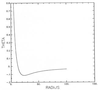
Fig. 1. Graph of θ (Eq. 18) for β=.5 and τ=100.
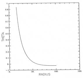
Fig. 2. Graph of θ (Eq. 18) for β=.5 and τ=1000.
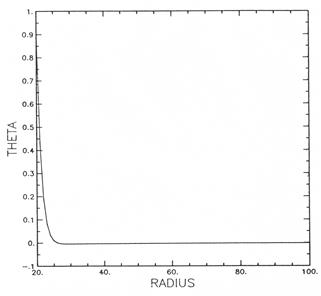
Fig. 3. Graph of θ (Eq. 18) for β=5. and τ=16.
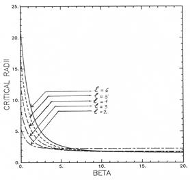
Fig. 4. Graph of Critical Radius for l=2 to 6.
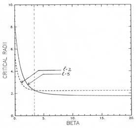
Fig. 5. Transition point between l = 2 & 3 modes.
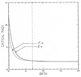
Fig. 6. Transition point between l = 3 & 4.
6. Conclusions
The purpose of the present work was to study the stability of solidifying spheres for intermediate rates of growth (i.e., β finite). This was done numerically and the results were compared to those obtained analytically in the limiting cases ![]() and
and![]() . Our results agreed with the theoretical work and moreover produced some unexpected conclusions. As opposed to the classical progression of instabilities predicted by the Mullins and Sekerka theory, we find that for large enough β the
. Our results agreed with the theoretical work and moreover produced some unexpected conclusions. As opposed to the classical progression of instabilities predicted by the Mullins and Sekerka theory, we find that for large enough β the ![]() -mode can lose stability before the
-mode can lose stability before the ![]() -mode. Indeed we find similar increasing transition values of
-mode. Indeed we find similar increasing transition values of ![]() for all pairs
for all pairs ![]() and
and![]() . This does not conflict with the Mullins and Sekerka theory which is valid only for
. This does not conflict with the Mullins and Sekerka theory which is valid only for![]() . This is also compatible with the finite-tome blow-up result of Chadam et al. [1] concerning spherical solutions. Our results indicate that the time of blow-up, the surface of the spherical solution undergoes quite complicated transitions, all modes being unstable simultaneously.
. This is also compatible with the finite-tome blow-up result of Chadam et al. [1] concerning spherical solutions. Our results indicate that the time of blow-up, the surface of the spherical solution undergoes quite complicated transitions, all modes being unstable simultaneously.
Acknowledgement
I am very grateful to Prof. Dr. John Chadam, for his critical comments and valuable advice throughout the course of research work. This research work was completed during M.Sc. from McMaster University, Canada in 1989.
References
- Chadam, J., Howison, S. D. and Ortoleva, P. (1987). IMA, Journal of Applied Math. 39, 1-15.
- Mullins, W. W. and Sekerka, R. F. (1963). Journal of Applied Physics. 34, 323-329.
- Mullins, W. W. and Sekerka, R. F. (1964). Journal of Applied Physics. 35, 444-451.
- Krukowski, S. and Turski, L. A. (1982). Journal of Crystal Growth. 58, 631-762.
- Chadam J. and Ortoleva, P. (1983). J. I. M. A. 30, 57-66.
- Chadam, J., Billon, J. C., Bertsch, M., Ortoleva, P. and Peletie, L. A. (1985), College de France Seminar Vol. VI Research Notes in Mathematics 109. Pitman, London.
- Chadam J. and Ortoleva, P. (1980). Proceedings of the Conference on Mathematical Biology, Carbondale, Illinois.
- Rubenstein, L. I. (1971). The Stefan Problem. Translations of Mathematical Monographs 27, AMS, Providence.
- Shafique, M. and Abbas, M. (1998) G. U. Journal of Research, 18, 89-94.
- Shafique, M. (1989). M.Sc. Thesis. McMaster University, Hamilton, Canada.
- Andrews, L. C. (1985). Special Functions for Engineers and Applied Mathematics, Macmillan Publishing Company, NY.
- Press, W. H., Flannery, B. P., Teukolsky, S. A. and Vetterling, W. T. (1986), Numerical Recipes. Cambridge University Press, Cambridge.
- Jones, W. B. and Thorn, W. J. (1980). Continued Fractions: Analytic Theory and applications, Addison-Wesley, Reading.
- Whittaker, E. T. and Watson, G, N. (1927). A course of modern analysis. University press, Cambridge.
- Abramowitz, M. and Stegun, I. A. (1964). Hand book of mathematical functions. U. S. Government printing office, Washington, D.C.
- Davis, P. J. and Rabinowitz, P. (1984). Methods of Numerical Integration. Academic Press, Inc.
- Carslaw, H. S. and Jaeger, J. C. (1959). Conduction of Heat in Solds. Clarendon, Oxford
- Friedman, A. (1964). Partial Differential Equations of Parabolic Type, Prentice-Hall, Englewood Cliffs.
- Friedman, A. (1982). Variational Principles and free Boundary Problems. Wiley, New York.
- Elliott, C. M. & Ockkendon, J R. (1982). Weak and Variation methods for moving boundary problems. Pitman, London.


