B-splines Method with Redefined Basis Functions for Solving Barrier Options Pricing Model

J. Rashidinia, Sanaz Jamalzadeh^*

School of Mathematics, Iran University of Science & Technology, Narmak, Tehran, Iran

Abstract

In this paper, we construct a numerical method to the solution of Black-Scholes partial differential equation modelling Barrier option pricing problem on a single asset. We use finite difference approximations for temporal derivative and then the option price is approximated with the redefined B-spline functions. Stability of this method has been discussed and shown that it is unconditionally stable. The developed method is tested on down-and-out Barrier problem and the numerical results are reported in tabular form where approximation solutions are compared with exact ones. They show the numerical results are in good agreement with exact solutions.

Keywords

Options Pricing, Redefined Cubic B-spline, Stability

Received: March 16, 2015
Accepted: April 2, 2015
Published online: April 6, 2015

@ 2015 The Authors. Published by American Institute of Science. This Open Access article is under the CC BY-NC license. http://creativecommons.org/licenses/by-nc/4.0/

1. Introduction

An option is a contract between two parties about trading the asset at a certain future time. One party is the writer, for example, a bank, who fixes the terms of the option contract and sells the option. The other party is the holder, who purchases the option, paying the market price, which is called premium. Options have a limited life time. The maturity date  fixes the time horizon. At this date the rights of the holder expire, and for later times () the option is worthless.There are two basic types of option: call and put. The call option gives the holderthe right to buy the underlying for an agreed price E by the date . The putoption gives the holder the right to sell the underlying for the price  by the date. The previously agreed price  of the contract is called strike or exercise price.Options with the barrier feature are considered to be the simplest types ofpath dependent options. Barrier options distinctive feature is that the payoff depends not only on the final price of the underlying asset, but also on whether the asset price has breached (one-touch) some barrier level during the life of the option.

Barrier options can be classified into knock-out and knock-in options. Assuming that the barrier price is , the knock-out option can be exercised unlessthe asset price  reaches the barrier  during the day of purchase and expirationday. The knock-in option can be exercised if the asset price  overtakes the barrier. The knock-out options can be classified into up-and-out and down-and-out. The up-and-out option can be exercised unless the asset price  reaches the barrier from below the barrier and the down-and-out option can be done unless theasset price reaches the barrier from above the barrier. The knock-in options can be classified into up-and-in and down-and-in. The up-and-in option can be exercised if the asset reaches the barrier from below the barrier whereas the down-and-in option can be exercised if the asset price reaches the barrier from above the barrier [1].

Option pricing theory has made a great leap forward since the development of the Black-Scholes option pricing model by Fischer Black and Myron Scholes in [2],and by Robert Merton in [3]. In an idealized financial market the price of Barrier options, is governed with Black-Scholes equation. We consider the dividend-free Black-Scholes equation,

(1.1)

where  is the option price,  is the risk free interest rate,  the volatility and  the stock price, associated with a final condition  and boundary conditions of the form,

(1.2)

where is the expiry time, we consider a truncated domain Following [4], a simple transformationchanges the Black-Scholes equation into a constant-coefficient  in the domain,

(1.3)

with the final condition  and boundary conditions,

(1.4)

As far as the relevant research in this direction is concerned, we mention that Figlewski and Gao [5] illustrated the application of an adaptive mesh technique to the case of barrier options. Zvan et al. [6], proposed to use an implicit method which has superior convergence (when the barrier is close to the region of interest)and stability properties as well as offering additional flexibility in terms of constructing the spatial grid. For some further reading on Barrier options, the reader may refer to [7-18].

The rest of the paper is organized as follows. In Section 2, we present a finite difference approximation to discretize equation (1.3) in time variable. The B-spline collocation method is constructed in Section 3. This method is analysed for stability in Section 4. Comparative numerical results are presented in Section 5.

2. Description of Method

We consider a uniform mesh  with the grid points  to discretize the region Eachis the vertices of the grid points, where and

Our numerical treatment for solving equation (1.3) using the collocation method with redefined cubic B-splines is to find an approximate solution  to exactsolution  in the form,

                    (2.1)

Where  are unknown time dependent parameters need to be determined.

Using approximate solution (2.1) and cubic B-spline, the approximate values at the knots of  and its derivatives are determined in terms of the time dependentparameters  as,

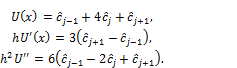(2.2)

We define the cubic B-spline for  by the following relationin [19] as,

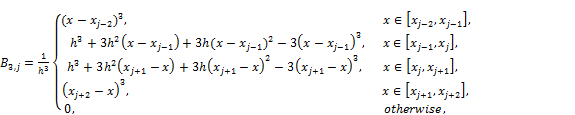(2.3)

Using (2.2) and boundary conditions (1.4), the approximate solutions at the boundary points are in the form,

               (2.4)

and,

            (2.5)

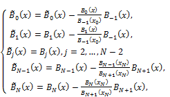
Following [20] the procedure for redefining the basis functions is as follows: Our numerical treatment for solving equation (1.3) with (1.4) using the Cubic B-splines collocation method with redefined basis functions is to find an approximate solution to the exact solution  by eliminating and from (2.1), (2.4) and (2.5); we get the approximate solution in the form,

(2.6)

where,

(2.7)

        (2.8)

Here the new set of basis functions isand they vanish on the boundary. The function  defined in (2.7) takes care of Dirichlet type boundary conditions. Applying the redefined set of basis functions into equation (1.3) we get the required approximate solution.

To apply the proposed method we discretize the problem in time variable using the backward finite difference approximation and the Crank-Nicolson scheme to space derivatives, we get,

(2.9)

Substituting the approximate solution  we have,

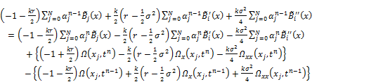(2.10)

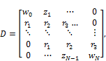
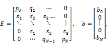
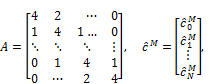
Substituting the approximate solution  and its derivatives and applying boundary conditions on (2.10), it can be written in matrix form as,

(2.11)

Where,

Now  and  are tri-diagonal matrices, which depends on boundary conditions. At each time level we solve (2.11) and recover the solution via(2.1).

3. Stability Analysis

We have established the stability analysis of the proposed method by using Von-Neumann stability method [20]. For stability analysis we should consider the equation (2.10) as follows,

(3.1)

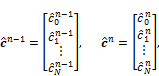
Now, it is necessary to assume that the solution of the scheme (3.1) at the mesh pointmay be written aswhere is, in general, complex, is themode number,  is the element size, and . Thus using in (2.12) we obtain the characteristic equation,

                 (3.2)

substituting the values of ,, , , ,and from (2.11) we have,

  (3.3)

                           (3.4)

where,

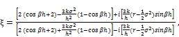
Now substitute ,  and  in equation (3.4) we have,

     (3.5)

so,

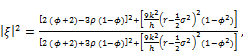         (3.6)

This implies, which is the condition for scheme to be unconditionally stable.

4. Final State

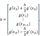
The Final vector can be determined from the Final condition which gives equations in  unknowns. For the determination of the unknowns,relations at the knot are used,

The final vector is then determined as the solution of the matrix equation,

5. Option Pricing Example

In this section, we shall consider the down-and-out option with the exercise price and the barrier . The option becomes invalid if the asset price  reaches thebarrier  from above the barrier during the day of purchase and the expiration date. Unless the asset price  reaches the barrier , i.e., , the option is aEuropean call option.

The value of the down-and-out option, denoted by  is governed by the equations,

where is the current value of the underlying asset at time  and  is the Barrier value. The final condition on the expiration day is given by,

and the boundary conditions are as follows,

In the case of Barrier options the first boundary condition is applied at rather than . If reaches , the option is invalid, thus on the line the value of the option is zero.Now we want to price the down-and-out call options with , ,,  and Barrier value . The analytical solution is given in [19].The comparison results with the exact solution is given in Table 1 with and .

Table 1. Comparison of results for down-and-out call option.

As it is seen from the tabular results, the B-spline approach gave the results which are in good agreement with the exact solution. Other types of Barrier options can similarly be solved but with different Final and boundary conditions.

Notations and Symbols‎‎

T: M‎aturity‎ time

‎E:‎ S‎tike ‎‎(‎exercise‎) ‎price

‎‎X:‎‎ Barrier ‎price

‎‎S: Asset price

‎V: Option price

‎‎:‎‎ Volatility

: Uniform mesh

‎U:‎ Approximate solution

‎u: ‎E‎xact‎ solution

‎: Cubic B-spline functions

‎(t): Time-dependent parameters

 Redefined cubic B-spline functions

‎ Mode number

‎h: ‎‎E‎lement ‎size

‎g(x): Final ‎condition

‎‎ First boundary condition

: Last boundary condition

‎‎ Grid ‎points

References

1. M.‎H.‎M.‎Khabir,‎Numerical singular perturbation approaches based on spline approximation methods for solving problems in computational‎finance,‎PhD thesis, University of the Western‎Cape,‎(2011).‎‎
2. F. Black, M. Scholes, The pricing of options and corporate liabilities, J. Polit,‎Econ‎81‎(3)‎,‎(1973)‎637-65‎4‎‎.‎
3. R. C. Merton, Theory of rational option pricing, Bell J. Econ‎4(1)‎,‎(1973)‎141-183‎.‎‎
4. A.‎Pena,‎Option Pricing with Radial Basis Functions: A‎Tutorial‎, Uni credit Banca Mobiliare SpA (UBM), 95 Gresham Street, London EC2V 7PN,‎UK.‎
5. ‎S. Figlewski and B. Gao, The adaptive mesh model: a new approach to efficient option pricing,‎J.‎Financ.‎Econ‎‎‎‎53‎,‎(1999) 313–351‎.‎
6. ‎R. Zvan, K.R. Vetzal and P.A. Forsyth, PDE methods for pricing barrier options,‎J.‎Econ.‎Dyn.‎Control‎‎‎24‎,‎(2000‎)‎1563–1590‎.‎
7. ‎M. Broadie, P. Glasserman and S. Kou, A continuity correction for discrete barrier options,‎Math.‎Finance 7(4)‎,‎(1997‎)‎325–348‎.‎
8. M. Broadie, P. Glasserman and S. Kou, Connecting discrete and continuous path dependent options, Finance‎Stochast‎3‎,‎(1999‎)‎55–82‎.‎
9. ‎P. Hörfelt, Pricing Discrete European Barrier Options using Lattice Random Walks,‎Math.‎Finance‎13(4)‎,‎(2003‎)‎503–524‎.
10. C.H. Hui, Time-Dependent Barrier Option Values,‎J.‎Futures.‎‎Market‎17(6)‎,‎(1997) 667–688‎.‎
11. Y. Lai, K. Lee, F. Chou and P. Chen, The Pricing Model of Discrete Barrier Options,‎Int.‎J.‎Financ.‎Econ 35‎,‎(2010) 1450–2887‎.‎‎
12. C. Lo, H. Lee and C. Hui, A simple approach for pricing barrier options with time-dependent parameters,‎Quant.‎‎Finance‎3‎,‎(2003) 98–107‎.
13. ‎S. Sanfelici, Galerkin infinite element approximation for pricing barrier option sand options with discontinuous payoff,‎Decis.‎Econ.‎‎Finance‎27‎,‎(2004) 125–151‎.‎‎
14. ‎M.A. Sullivan, Pricing discretely monitored barrier options,‎J.‎Comput.‎‎Finance‎3‎,‎(2000) 35–52‎.‎‎
15. B.A. Wade, A.Q.M. Khaliq, M. Yousuf, J. Vigo-Aguiar and R. Deininger, On smoothing of the Crank–Nicolson scheme and higher order schemes for pricing barrier options,‎J.‎Comput.‎Appl.‎‎Math‎204‎,‎(2007)144–158‎.‎‎
16. ‎J.Z. Wei, Valuation of discrete barrier options by interpolation,‎JOD‎6‎,‎(1998)‎‎51–73‎.
17. Z. Cen, A. Le, A robust and accurate finite difference method for a generalized Black-Scoles equation, J. Comput. Appl. Math. 235 (2011) 3728-3733.
18. J. Ahn, S, Kang, Y. Kwon, A Laplace transform finite difference method for the Black-Scholes equation, Math. Comput. Modelling, 51 (2010) 247-255.
19. ‎P. M. Prenter, Spline and Variational Methods, Wiley, New york,‎(‎1975‎)‎.‎‎‎
20. R.C. Mittal, R.K.‎Jain,‎Redefined cubic B-splines collocation method‎‎for solving convection–diffusion‎equations,‎Appl.‎Math.‎‎Model‎36, (2012) 5555-5573.
21. ‎P.‎Wilmott, Derivatives: The Theory and Practice of Financial Engineering. John Wiley & Sons, New‎York,‎(1998).‎