
International Journal of Mathematics and Computational Science, Vol. 1, No. 2, April 2015 Publish Date: Mar. 25, 2015 Pages: 30-36
Application of Level Set Method for Simulating Kelvin-Helmholtz Instability Including Viscous and Surface Tension Effects
Ashraf Balabel*
Mechanical Engineering Dept., Taif University, Taif, Hawiyya, Kingdom of Saudi Arabia
Abstract
In the present paper, the hydrodynamic instability known as Kelvin-Helmholtz instability is numerically investigated with the application of the level set method. First, the classical Kelvin-Helmholtz instability, which is concerned with the topological changes of interface separating two immiscible, incompressible and inviscid fluids (normally liquid/gas) in irrotational and relative motion, is predicted. Further, as in real flow, the effects of viscosity and surface tension are included. The numerical strategy is based on the solution of Navier-Stokes equations over a regular and structured two-dimensional computational grid using the control volume approach in both phases with a separate manner. The kinematic and the dynamic boundary conditions between the two phases are applied on the interface. The transient evolution of the interface due to the different surface forces is predicted by the level set method. The obtained results showed that the roll-up mechanism starting at the interface is largely affected by the different flow regimes considered. The inclusion of the viscous force can lead to a weakened roll-up mechanism. Moreover, the finite surface tension force can prevent the roll-up mechanism compared with classical Kelvin-Helmholtz instability.
Keywords
Kelvin-Helmholtz Instability, Level Set Method, Numerical Simulation, Surface Tension, Two-Phase Flow
Received: March 7, 2015
Accepted: March 20, 2015
Published online: March 23, 2015
@ 2015 The Authors. Published by American Institute of Science. This Open Access article is under the CC BY-NC license. http://creativecommons.org/licenses/by-nc/4.0/
1. Introduction
Many of industrial and engineering applications encounter a large number of two phase flows; e.g. atomization of liquid jets [1], droplet dynamics [2], bubble flow [3], and other multiphase flow systems [4].
The nonlinear stability of an interface between two incompressible, inviscid and irrotational fluids containing a velocity discontinuity remains a considerable challenge to mathematicians and numerical analysts. Helmholtz [5] was the first to remark on the instability of those interfaces. Kelvin [6] has discussed the conditions under which a plane surface of water becomes unstable. As a result of the velocity discontinuity presented initially in the flow, a vortex flow is produced and the motion of the interface is subjected to a well-known Kelvin-Helmholtz instability (KHI).
The basic mechanism of KHI development is in the existence of a uniform velocity shear between two different fluids. In most cases, the surface tension and viscosity are neglected in order to simplify the theoretical and numerical calculations and, consequently, KHI is considered as a fluid instability that a lighter fluid is superposed on a heavier one. The including of the gravity force or the density stratification, without any uniform shear considered, leads to the well known cases of Rayleigh-Taylor Instability or Richtmyer-Meshkov Instability.
The attention of KHI has received is due to in part to their importance as models of free shear layers in high Reynolds number flows. This, in turn, determines the rate of mixing in the flow. On the other hand, and based on the experimental observation, the interfacial roll-up is a prelude to drop formation in free surface flow evolution. The motion of the interfaces subjected to the vortex flows is widely investigated by means of different numerical methods; see for example [7,8].
In real systems, the interface is a layer with a finite thickness; in addition, viscosity or surface tension affects the interface evolution. The effect of viscosity on the evolution of KHI can be seen in suppressing the short-wave disturbance and in thickening the vortex sheet. It means that the roll-up was weakened by viscosity effects and the viscosity force acts as a regularization effect on the roll-up of vortex sheets.
The singularity formation is one of the most interesting phenomenons in the simulations of free surface flows and it is considered disastrous from the stand point of the numerical computations. In the absence of the surface tension, an appearance of a saw-tooth-like instability in the interface profiles has been observed. This instability prevents the simulations from proceeding to the late time highly nonlinear phase of the motion as singularities can form on the interface in finite time [7].
However, the inclusion of the surface tension effect was found to prevent the appearance of the numerical instability but only for finite times. Thereafter, locally irregular behavior eventually reappeared and resisted subsequent attempts at numerical smoothing. These irregularities are developed on the interface profile where some form of coherent roll-up might be expected. Although several numerical and/or physical mechanisms are discussed that might produce irregular behavior of the discretized interface in the presence of the surface tension term, the basic cause of this instability remains unknown.
According to [8], there is no published analytic study that has demonstrated that the surface tension effect removes the ill-posedness of the vortex sheet motion in both the linear theory and the nonlinear case. Furthermore, a saw-tooth-like instability that appeared in the solution, generally growing rather more rapidly in cases involving finite surface tension term. After greater values of time, the interface did not roll up smoothly but rather developed irregularities on the interface.
According to the experimental complexity of such problem, exact measurements of the interface shapes are not available; however, the theoretical as well as the numerical treatments of the Kelvin-Helmholtz instability have encountered some constraints related to the nature of the problem as it includes a transient, non-uniform free surface flow with large spatial and temporal gradients.
As a result of the huge development in the numerical simulation of two-phase flows, carefully executed simulations in such context can virtually replace experiments [9]. In general, the numerical predictions of two-phase flow dynamics have been limited in accuracy partly by the performance of three key elements, viz.: development of the computational algorithm, interface tracking methods, and turbulence prediction models [10].
A variety of numerical methods have been recently developed and validated to two-phase flow. However, an efficient and complete numerical method is not available. An extended review of numerical techniques applied for two-phase flow including adv/disadvantages can be found in [11].
More recently, the author has developed a new numerical method, known as Interfacial Marker Level Set Method (IMLS), for predicting the complete dynamics of two-phase flows. This numerical method is validated and its accuracy is estimated through the performing of a wide range of industrial and engineering applications [12-18]. This method is also further applied in the present paper and shortly explained in the following sections.
2. Computational Domain
Consider the two-dimensional motion of two immiscible, incompressible, inviscid fluids of equal density separated by an interface. The rectangular coordinates (x,y) have been chosen, with the x-axis horizontal and aligned with the initial mean level of the interface, and the y-axis vertical to it. The interfacial shape is assumed to be periodic in the x-direction with wavelength. The motion of the two fluids can be described in terms of the motion of a single wavelength of the interface. The fluid above the x-axis moves at a uniform velocity U, and below at uniform velocity of equal magnitude but in the opposite direction, as shown in Fig.(1).
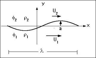
Figure 1. Configuration of the surface discontinuity
At time=0, the surface configuration can be considered as:
![]()
where a is the disturbance amplitude.
3. Mathematical Formulations
The governing equations for incompressible two-phase flow are mathematically expressed by the conservation equations of the mass and momentum at each point of the flow field. These equations can be written in the primitive variables formulation in form of continuity equation and Navier-Stokes equations, respectively, as follows:
![]() (1)
(1)
![]() (2)
(2)
where r, u, p, m are the density, velocity vector, pressure and viscosity of the fluid. The subscript i denotes the liquid phase (i=1) and the gas phase (i=2), respectively. It is known that, for two–phase flows, the pressure and velocity field are caused by the external gas stresses in the tangential and normal directions. Therefore, the dynamic balance between both phases can be obtained by solving the complete set of the governing equations in the gas phase for the velocity and pressure for the gas phase surface and using these values as boundary conditions for solving the interior of the liquid phase to specify the exact level of pressure and velocity components inside it. The obtained normal velocity component at the liquid interface is then used to obtain the topological changes and deformation of the droplet surface via the level set method.
The fact that there is no pressure transport equation necessitates the consideration of the continuity equation as a means to obtain the correct pressure field. This is done by a proper coupling between the pressure and velocity field through the Poisson equation for pressure:
![]() (3)
(3)
The Poisson equation is solved by means of the Successive Over-Relaxation method in each phase to obtain the pressure level inside the considered phase.
In our algorithm, the implicit fractional step-non iterative method is applied to obtain the velocity and pressure filed by presuming that the velocity field reaches its final value in two stages; that means
![]() (4)
(4)
whereby, ![]() is an imperfect velocity field based on a guessed pressure field, and
is an imperfect velocity field based on a guessed pressure field, and ![]() is the corresponding velocity correction. Firstly, the 'starred' velocity will result from the solution of the momentum equations. The second stage is the solution of Poisson equation for the pressure:
is the corresponding velocity correction. Firstly, the 'starred' velocity will result from the solution of the momentum equations. The second stage is the solution of Poisson equation for the pressure:
![]() (5)
(5)
where ![]() will be called the pressure correction. Once this equation is solved, one gets the appropriate pressure correction, and consequently, the velocity correction is obtained according to:
will be called the pressure correction. Once this equation is solved, one gets the appropriate pressure correction, and consequently, the velocity correction is obtained according to:
![]() (6)
(6)
This fractional step method described above ensures the proper velocity-pressure coupling for incompressible flow fields.
3.1. Interfacial Boundary Conditions
The boundary conditions at the interface, or jump conditions, are comprised of the dynamic and kinematic conditions. In the case of two immiscible fluids, referring to Fig.2, the dynamic stress balance at the liquid interface G may be written in the following general form:
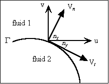
Figure 2. Normal and tangential velocity components of an arbitrary interface
![]() (7)
(7)
where I is the identity matrix, p is the pressure, m is the dynamic viscosity, s is the surface tension coefficient, and D is the rate of deformation tensor. The bracket means the jump of the stresses along the fluid interface G, the unit normal vector n is taken from fluid 2 to fluid 1,![]() denotes the gradient in the local free surface coordinates, and t is an arbitrary vector perpendicular to the normal of the interface. The curvature of the interface k is computed from the following equation:
denotes the gradient in the local free surface coordinates, and t is an arbitrary vector perpendicular to the normal of the interface. The curvature of the interface k is computed from the following equation:
![]() (8)
(8)
The normal and tangential velocity components are Vn and Vt respectively. It is clear that, the effect of the surface tension is to balance the jump of the normal stress along the fluid interface. The second term on the right hand side of the dynamic stress equation, Eq.(7), is the stress due to the gradient on surface tension in the local interface coordinates or the so-called Marangoni effect, usually important when a temperature gradient is applied parallel to the interface, e. g. thermocapillary convection.
In contrast to the previous two-phase numerical methods, in which the interfacial jump conditions are embedded naturally on the momentum equations by applying CSF model [19], the jump conditions between the two fluids are treated here as a boundary conditions enforced explicitly at the interface G. Taking the projections of the jump conditions in the directions normal and tangential to the interface, considering a constant surface tension, one obtains the following two equations in the normal and tangential directions, respectively:
![]() (9)
(9)
![]() (10)
(10)
It is noticed from the above equations that surface tension effects are included in the normal stress balance, while the equality of the shear stress is satisfied in the tangential direction. In the special case of inviscid flow with constant surface tension coefficient the above equations are reduced to the Young-Laplace equation which determines the pressure jump across the interface.
In addition to the equality of the dynamic interfacial stresses described above, the kinematic conditions should also be considered. When there is no mass transfer through the interface, the kinematic conditions is satisfied by assuming the continuity of the normal velocity components, i.e.
![]() (11)
(11)
In addition to that, the liquid gas interface requires equality of dynamic stresses, especially shear stresses, on both sides of the interface, i.e.
![]() (12)
(12)
The system of the above equations and the prescribed boundary conditions should be solved simultaneously to determine the flow field in the two fluids. The normal velocity components are then used for the advection of the interface by solving the appropriate equation of the level set function.
3.2. Level Set Function
The level set method is a type of capturing methods where a defined phase function f, is smoothed over the entire computational domain. The level set function at any given point is taken as the signed normal distance from the interface with positive on the liquid phase (i.e. f>0), and negative on the gas phase (i.e. f<0). Consequently, the interface is implicitly defined as the zero level set of the level set function.
The transport equation of the level set function can be described by the following equation:
![]() (13)
(13)
where ![]() is the velocity vector. The geometrical properties of the interface, (normal vectors and curvature), can be defined as:
is the velocity vector. The geometrical properties of the interface, (normal vectors and curvature), can be defined as:
![]() (14)
(14)
The original work of level set method in two-phase numerical simulation is referred to [20]. A review of such works can be found in the cited review [16].
3.3. Computational Methodology
In order to solve the above system of equations, the prescribed control volume formulation presented by [21] has been implemented. However, according to the complexities introduced by the staggered grid system in two-phase flow calculations and the need to track the liquid surface, a non-staggered grid system is applied here, which requires the use of a single cell network for all variables and a collocated specification of variables at the centre of each cell.
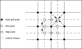
Figure 3. Calculation stencil for obtaining the intermediate flux velocity at cell faces
The collocated specifications of flow variables require a spatial technique to prevent pressure decoupling between adjacent cells. The only drawback of the non-staggered grid system is that it requires a high-order approximation for calculation of the fluxes and to obtain difference equations that can prevent pressure oscillations. In the present study, the derivatives at the central point of the control volume are approximated using the second-order central difference scheme to achieve the best accuracy. The velocity components at the control volume faces are calculated using the average values of the two-edge points that are calculated through the average of the four neighbouring grid points, as seen in figure 3.
3.4. Initial Complex Velocity Field
In order to start the calculation, a velocity field has to be prescribed. The initial velocity field plays a significant role in the properly started calculations, and consequently in the physical deformation of the interface. In KHI, a complex velocity field can be obtained through a distribution of vortex-like singularities on the interface [22]. The velocity components induced at point p located at the centre of the computational domain.
![]()
![]()
where N is the number of the vortices on the interface. In the present work only one vortex pole located at the center of the computational domain.
4. Results and Discussion
In the present section, three different cases with the data shown in Table 1 are performed. The first case is performed for zero surface tension and zero viscosity fluids, while the other cases are performed by including the viscosity and surface tension respectively.
Table 1. Data for the performed test cases
| Property | ρ1/ ρ2 | μ1/ μ2 | σ (N/m) | Grid | Δx, Δy | Δt |
| Case I | 1.0 | 0.0 | 0.0 | 151x151 | 1e-4, 1e-4 | 3e-7 |
| Case II | 1.0 | 1.0 | 0.0 | 151x151 | 1e-4, 1e-4 | 3e-7 |
| Case III | 1.0 | 1.0 | 0.001 | 151x151 | 1e-4, 1e-4 | 3e-7 |
4.1. Case I
The evolution of an initial sinusoidal disturbance with amplitude a = 0.06l is shown in Fig.(4). It is clear that the proper initial velocity distribution produces a good behaved smooth roll-up and concentration of vorticity at the midpoint of the wavelength (x =l/2). No singularities can be observed. The roll-up process agrees well with the previous expectations [22,23], and the interface forms at later times a smooth spiral.
In comparison with the results [24], the proposed numerical procedure can properly predict the evolution of the interface without any numerical problems. That reveals the effectiveness of the numerical method adopted in order to obtain a real physical phenomenon.
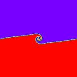
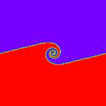
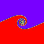
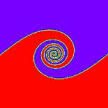
Figure 4. Evolution of KHI for Case I
4.2. Case II
In order to show the effect of viscous force on the evolution of the KHI, the previous test case (Case I) is performed, however, the viscosity term is included in the governing equations with a viscosity ratio between the two fluids equal 1. The inclusion of the viscosity effect in two-phase simulations is normally a challenge task due to the existence of the interfacial viscous stresses and the difficulties associated with its numerical modelling.
From Fig. 5, it can be seen that the viscosity acts to thicken the vortex sheet and tries to suppress the roll-up mechanism observed in the inviscid simulations. The numerical results obtained for the viscous simulation predict that viscosity acts as a regularization effect on the roll-up of vortex sheets. These observations coincide with the previous investigations [24].
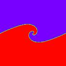
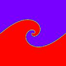
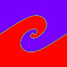
Figure 5. Evolution of KHI for Case II
4.3. Case III
In the present section, the effect of the finite surface tension on the rolling-up mechanism of the initial wave disturbance is presented, while the viscous effects are neglected. By including the finite surface tension into the numerical simulation, it is observed that the roll-up can occur as shown in Fig. 6. However, it can be observed a phenomenon called "pinching singularity" in contrast to the roll-up mechanism for case I. Moreover, the rolling-up mechanism in case of finite surface tension is weakened in comparison with the results of Case I.
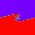
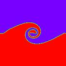
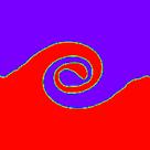
Figure 6. Evolution of KHI for Case III
5. Conclusion
The present paper investigates numerically the known Kelvin-Helmholtz instability between two fluids with different flow regimes. The numerical simulation is carried out by solving Navier-Stokes equations coupled with level set method in both fluids. The interfacial boundary conditions are well described in both fluids. The results indicate that, in case of inviscid simulation the roll-up mechanism of the interface separating the two fluids is well predicted. By including the viscosity effect in the numerical simulation, the roll-up mechanism is weakened. The effect of including the surface tension can be seen in observing the pinching singularity phenomenon called in contrast to the roll-up mechanism for inviscid flow. In general, the applied numerical method is seen to be effective and robust in two-phase flow simulations.
References
- Lefebvre, A. H. (1989): Atomization and sprays, Hemisphere Publishing Corporation.
- Fuster, D., Agbaglah, G., Josserand, C., Popinet, S. and Zaleski, S. (2009): Numerical simulation of droplets, bubbles and waves: state of the art, Fluid Dyn. Res. 41, 1-24.
- Sato, Y. (1975): Liquid velocity distribution in two phase bubble flow, Int. J. Multiphase flow, vol. 2(1), pp. 79-95.
- Kolev, N.I., (2007): Multiphase flow dynamics: Thermal and Mechanical Interaction", Springer.
- Helmholtz, H., Ueber Discontinuirliche Fluessigkeitsbewegungen. Monatberichte Akad. d. Wiss. Berlin, vol.23, pp.215-228, 1868.
- Kelvin, L. Mathematical and Physical Papers, vol. 4, pp.76-100, 1910.
- D. I. Pullin. Numerical Studies of Surface-Tension Effects in Nonlinear Kelvin-Helmholtz and Rayleigh-Taylor Instability. J. Fluid Mech., vol.119, pp.507-532, 1982.
- M. Siegel. A Study of Singularity formation in the Kelvin-Helmholtz Instability with Surface Tension. Siam J. App. Math., vol.55, No.4, pp. 865-891, 1995.
- Eggers, J. Nonlinear Dynamics and Breakup of Free-Surface Flow, Rews. Modern Phys., vol. 69, No. 3, pp. 865–929, (1997).
- Balabel A. Numerical Modelling of Liquid Jet Breakup by Different Liquid Jet/Air Flow Orientations Using the Level Set Method, Computer modeling in engineering & sciences, vol. 95 (4), pp. 283-302, (2013).
- Shinjo J. and Umemura A., (2010): Simulation of liquid primary breakup: Dynamics of ligament and droplet formation", Int. J. Multiphase Flow, vol. 36(7), pp. 513-532.
- Balabel, A.; El-Askary, W. On the performance of linear and nonlinear k–e turbulence models in various jet flow applications. European Journal of Mechanics B/Fluids, vol. 30, pp. 325–340, 2011.
- Balabel, A. Numerical prediction of droplet dynamics in turbulent flow, using the level set method. International Journal of Computational Fluid Dynamics, vol. 25, no. 5, pp. 239-253, 2011.
- Balabel, A. Numerical simulation of two-dimensional binary droplets collision outcomes using the level set method. International Journal of Computational Fluid Dynamics, vol. 26, no. 1, pp. 1-21, 2012.
- Balabel, A. Numerical modeling of turbulence-induced interfacial instability in two-phase flow with moving interface. Applied Mathematical Modelling, vol. 36, pp. 3593–3611, 2012.
- Balabel, A. A Generalized Level Set-Navier Stokes Numerical Method for Predicting Thermo-Fluid Dynamics of Turbulent Free Surface. Computer Modeling in Engineering and Sciences (CMES), vol.83, no.6, pp. 599-638, 2012.
- Balabel, A. Numerical Modelling of Turbulence Effects on Droplet Collision Dynamics using the Level Set Method. Computer Modeling in Engineering and Sciences (CMES), vol. 89, no.4, pp. 283-301, 2012.
- Balabel, A, El-askary, W., Wilson, S. Numerical and Experimental Investigations of Jet Impingement on a Periodically Oscillating-Heated Flat Plate. Computer Modeling in Engineering and Sciences (CMES), vol. 95 (6), pp. 483-499, 2013.
- Brackbill, J. U., Kothe, D. B. and Zemach. A. A Continuum Method for Modeling Surface Tension, J. Comp. Physics, 100, 335-354, 1992.
- Sussman, M., Smereka, P. and Osher, S. A level set approach for computing solutions to incompressible two-phase flows, J. Comp. Physics, 114, 146-159, 1994.
- span>Patankar, S. V., Numerical Heat Transfer and Fluid Flow. Hemisphere Publishing Corporation, 1980.
- D. I. Pullin. Numerical Studies of Surface-Tension Effects in Nonlinear Kelvin-Helmholtz and Rayleigh-Taylor Instability. J. Fluid Mech., vol.119, pp. 507-532, 1982.
- J.L. Hans. Vortex Flow in Nature and Technology. John wiley and Sons, 1983.
- T. Hou, J. Lowengrub, and M. Shelley. Removing the Sti_ness form Interfcaial Flows with Surface Tension. J. comp. Phys., vol.114, pp.312-338, 1994.
- S-I. Sohn Singularity formation and nonlinear evolution of a viscous vortex sheet model Phys. Fluids 25 (1), p014106, 2013.


