
International Journal of Mathematics and Computational Science, Vol. 1, No. 2, April 2015 Publish Date: Mar. 26, 2015 Pages: 50-54
An Economic Reliability Test Plan Based on Truncated Life Tests for Marshall-Olkin Extended Weibull Distribution
G. Srinivasa Rao*
Department of Statistics, The University of Dodoma, Dodoma, Tanzania
Abstract
The Marshall-Olkin extended Weibull distribution is considered as a probability model for the lifetime of the product. A test plan to determine the termination time of the experiment for a given sample size, producer’s risk and termination number is constructed. The preferability of the present test plan over similar plans exists in the literature is established with respect to time of the experiment. Results are illustrated by an example.
Keywords
Marshall-Olkin Extended Weibull Distribution, Reliability Test Plan, Minimum Sample Size, Producer’s Risk
Received: March 6, 2015
Accepted: March 25, 2015
Published online: March 26, 2015
@ 2015 The Authors. Published by American Institute of Science. This Open Access article is under the CC BY-NC license. http://creativecommons.org/licenses/by-nc/4.0/
1. Introduction
The two important tools for ensuring quality are the statistical quality control and the acceptance sampling. The acceptance sampling is a sampling inspection in which the consumer decides to accept or to reject a lot of products shipped by the producer, based on the results of a random sample selected from that lot. An acceptance sampling plan is a specific plan that establishes the minimum sample size to be used and the associated acceptance and non-acceptance criteria for the lot. In this kind of tests we put n items on the test. We pre-assigned the values of t and c (acceptance number for this experiment). If the number of failures is greater than c, this leads the decision to reject the lot of product. In life test, one may wait until c failures occur or time is ended. Using life test one may find the probability of acceptance, minimum sample size put on the test and the minimum ratio of true average life to the specified average life or quality level subject to the consumer’s risk. The life tests of this type for various non-normal situations are developed by Epstein (1954), Sobel and Tischendr of (1959), Goode and Kao (1961),Gupta and Groll (1961), Gupta (1962), Kantam et al. (2001, 2006), Baklizi (2003), Tsai and Wu (2006), Balakrishnan et al. (2007), Aslam and Shahbaz (2007), Aslam and Kantam (2008), Rao et al.(2008, 2009a, 2009b), Sriramachandran and Palanivel (2014) and Priyah and Sudamani (2015). The purpose of this paper is to find the termination time assuming the Marshall-Olkin extended Weibull distribution as a life time model. Comparison of the proposed reliability plan has been made with the acceptance sampling plan developed by the Rao and Rao (2012) for Marshall-Olkin extended Weibull distribution. We give a brief presentation of Rao and Rao (2012) followed by the construction of sampling plan with a new approach in Section 2. The operating characteristic is presented in Section 3. The comparative studies of results are discussed with examples in Section 4.
2. Economic Reliability Sampling Test Plans
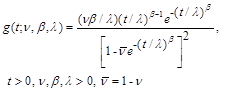
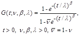
We assume that the lifetime of a product follows Marshall-Olkin extended Weibull distribution introduced by Marshall and Olkin (1997) and its applications to censored data are studied by Ghitany et al.(2005). The probability density function (p.d.f.) and cumulative distribution function (c.d.f.) of scaled Marshall-Olkin extended Weibull distribution are given by
 (2.1)
(2.1)
 . (2.2)
where![]() is the scale parameter and
is the scale parameter and![]() is shape parameter. Marshall-Olkin extended Weibull distribution.
is shape parameter. Marshall-Olkin extended Weibull distribution.
Consider a null hypothesis "![]() ". If Marshall-Olkin extended Weibull distribution is assumed as the model of a variable representing lifetimes of some items that have life and eventual failure, the above hypothesis is regarding the average life of those items in the population. If the
". If Marshall-Olkin extended Weibull distribution is assumed as the model of a variable representing lifetimes of some items that have life and eventual failure, the above hypothesis is regarding the average life of those items in the population. If the ![]() is accepted on the basis of some sample lifetimes collected through a life testing experiment from out of a submitted lot of such items using any admissible statistical test procedure, we may conclude that the submitted lot has a better average life than what is specified accordingly the lot that can be termed as a good lot and can be accepted. Rao and Rao (2012) constructed the minimum sample size required to make a decision about the lot given the waiting time in terms of
is accepted on the basis of some sample lifetimes collected through a life testing experiment from out of a submitted lot of such items using any admissible statistical test procedure, we may conclude that the submitted lot has a better average life than what is specified accordingly the lot that can be termed as a good lot and can be accepted. Rao and Rao (2012) constructed the minimum sample size required to make a decision about the lot given the waiting time in terms of ![]() (i.e.,
(i.e.,![]() ) and acceptance number c, some risk probability, say
) and acceptance number c, some risk probability, say![]() . With a specified
. With a specified ![]() of
of![]() , the probability of detecting c or less failures (probability of accepting the lot) in a sample of size n is given by
, the probability of detecting c or less failures (probability of accepting the lot) in a sample of size n is given by
![]() , (2.3)
, (2.3)
where![]() .
.
For![]() , the above probability of acceptance should increase. Therefore, if
, the above probability of acceptance should increase. Therefore, if ![]() is a prefixed risk probability this means
is a prefixed risk probability this means
![]() . (2.4)
. (2.4)
For a given ![]() and hence of
and hence of ![]() , this is a single inequality in two unknowns n and c assuming that the parameters
, this is a single inequality in two unknowns n and c assuming that the parameters ![]() are known. Because, c is always less than n, inequality (2.4) can be solved for n with successive values of c from zero onwards. The earliest values of n satisfying the inequality (2.4) are given for
are known. Because, c is always less than n, inequality (2.4) can be solved for n with successive values of c from zero onwards. The earliest values of n satisfying the inequality (2.4) are given for![]() = 0.75, 0.90, 0.95, 0.99 and
= 0.75, 0.90, 0.95, 0.99 and ![]() =0.628, 0.942, 1.257, 1.571, 2.356, 3.141, 3.927, 4.712 for
=0.628, 0.942, 1.257, 1.571, 2.356, 3.141, 3.927, 4.712 for![]() by Rao and Rao (2012) along with the associated performance characteristics like operating characteristics, producer’s risk, scope for variability of
by Rao and Rao (2012) along with the associated performance characteristics like operating characteristics, producer’s risk, scope for variability of![]() etc.
etc.
In the present investigation, inequality (2.4) can be considered in a different way. Let us fix n and let r be a natural number less than n, so that as soon as the ![]() (r =c+1) failure is observed, the process is stopped and the lot is rejected. Given
(r =c+1) failure is observed, the process is stopped and the lot is rejected. Given![]() , the probability of such a rejection should be as small as possible. That is
, the probability of such a rejection should be as small as possible. That is
![]() . (2.5)
. (2.5)
Table 1. Life test termination time in units of scale parameter (![]() ) inMarshall-Olkin extended Weibull distribution for
) inMarshall-Olkin extended Weibull distribution for![]() .
.
|
|
|
|
|
|
|
|
|
|
|
|
| |||||||||
| 1 | 0.25124 | 0.20573 | 0.17861 | 0.16027 | 0.14647 | 0.13589 | 0.12639 | 0.11929 | 0.11394 |
| 2 | 0.48945 | 0.39386 | 0.33882 | 0.30203 | 0.27515 | 0.25417 | 0.23758 | 0.22418 | 0.21226 |
| 3 | 0.61085 | 0.48970 | 0.42076 | 0.37481 | 0.34134 | 0.31518 | 0.29461 | 0.27738 | 0.26324 |
| 4 | 0.68461 | 0.54802 | 0.47082 | 0.41931 | 0.38191 | 0.35298 | 0.32964 | 0.31046 | 0.29419 |
| 5 | 0.73462 | 0.58782 | 0.50500 | 0.44977 | 0.40962 | 0.37870 | 0.35367 | 0.33334 | 0.31596 |
| 6 | 0.77120 | 0.61711 | 0.53038 | 0.47236 | 0.43018 | 0.39756 | 0.37154 | 0.35019 | 0.33187 |
| 7 | 0.79948 | 0.63964 | 0.54978 | 0.48995 | 0.44625 | 0.41258 | 0.38541 | 0.36322 | 0.34420 |
| 8 | 0.82218 | 0.65777 | 0.56552 | 0.50404 | 0.45910 | 0.42450 | 0.39664 | 0.37384 | 0.35436 |
| 9 | 0.84074 | 0.67275 | 0.57834 | 0.51563 | 0.46953 | 0.43412 | 0.40574 | 0.38255 | 0.36255 |
| 10 | 0.85625 | 0.68531 | 0.58924 | 0.52536 | 0.47872 | 0.44270 | 0.41376 | 0.38982 | 0.36956 |
|
| |||||||||
| 1 | 0.11284 | 0.09216 | 0.08060 | 0.07244 | 0.06518 | 0.06123 | 0.05700 | 0.05476 | 0.05243 |
| 2 | 0.32249 | 0.25803 | 0.22140 | 0.19711 | 0.17930 | 0.16561 | 0.15474 | 0.14562 | 0.13771 |
| 3 | 0.45645 | 0.36322 | 0.31086 | 0.27649 | 0.25124 | 0.23178 | 0.21631 | 0.20392 | 0.19330 |
| 4 | 0.54383 | 0.43215 | 0.36989 | 0.32890 | 0.29876 | 0.27605 | 0.25755 | 0.24222 | 0.22964 |
| 5 | 0.60552 | 0.48124 | 0.41199 | 0.36624 | 0.33298 | 0.30728 | 0.28699 | 0.27018 | 0.25611 |
| 6 | 0.65173 | 0.51797 | 0.44352 | 0.39448 | 0.35848 | 0.33113 | 0.30927 | 0.29083 | 0.27560 |
| 7 | 0.68776 | 0.54692 | 0.46850 | 0.41669 | 0.37870 | 0.34984 | 0.32665 | 0.30768 | 0.29167 |
| 8 | 0.71686 | 0.57039 | 0.48871 | 0.43468 | 0.39540 | 0.36524 | 0.34098 | 0.32097 | 0.30406 |
| 9 | 0.74083 | 0.58965 | 0.50547 | 0.44977 | 0.40903 | 0.37773 | 0.35298 | 0.33224 | 0.31479 |
| 10 | 0.76125 | 0.60612 | 0.51983 | 0.46252 | 0.42076 | 0.38856 | 0.36289 | 0.34170 | 0.32401 |
Specifying n as a multiple of r say![]() , inequality (2.5) can be regarded as an inequality in a single unknown in terms of
, inequality (2.5) can be regarded as an inequality in a single unknown in terms of ![]() with
with![]() . With the choice of r, k,
. With the choice of r, k,![]() inequality (2.5) can be solved for the earliest p say
inequality (2.5) can be solved for the earliest p say ![]() from which the value of
from which the value of ![]() can be obtained by inverting the
can be obtained by inverting the ![]() given by (2.2). The specified population average in terms of
given by (2.2). The specified population average in terms of ![]() can be used here to get the value of t called the termination time. These are presented in Table1 for various values of n, r =1(1)10,
can be used here to get the value of t called the termination time. These are presented in Table1 for various values of n, r =1(1)10,![]() at
at ![]() =0.05 and 0.01.
=0.05 and 0.01.
3. Operating Characteristic Function
If the true but unknown life of the product deviates from the specified life of the product it should result in a considerable change in the probability of acceptance of the lot based on the sampling plan. Hence the probability of acceptance can be regarded as a function of the deviation of specified average from the true average. This function is called operating characteristic (OC) function of the sampling plan. The operating characteristic function of economic sampling plan![]() gives the probability of acceptance of the submitted lot of the product; this probability of acceptance is given by
gives the probability of acceptance of the submitted lot of the product; this probability of acceptance is given by
![]() (3.1)
(3.1)
The probabilities of acceptance given by equation (3.1) for a sampling plan forms the O.C. curve of that plan and are given in Table 2.
Table 2. Operating characteristic (O.C) values of sampling plans ![]() for
for ![]() .
.
|
|
|
|
|
|
|
|
|
|
|
|
| |||||||||
| 1 | 0.94984 | 0.94986 | 0.94977 | 0.94955 | 0.94950 | 0.94934 | 0.94993 | 0.94985 | 0.94920 |
| 2 | 0.94992 | 0.94993 | 0.94998 | 0.94993 | 0.94988 | 0.95000 | 0.94992 | 0.94960 | 0.94983 |
| 3 | 0.94997 | 0.94993 | 0.94995 | 0.94989 | 0.94980 | 0.95000 | 0.94984 | 0.94992 | 0.94963 |
| 4 | 0.94992 | 0.94994 | 0.94992 | 0.94990 | 0.94976 | 0.94972 | 0.94982 | 0.94983 | 0.94994 |
| 5 | 0.94995 | 0.94995 | 0.94996 | 0.94998 | 0.94989 | 0.94977 | 0.94990 | 0.94967 | 0.94972 |
| 6 | 0.95000 | 0.94992 | 0.94984 | 0.94994 | 0.94991 | 0.94997 | 0.94987 | 0.94964 | 0.94979 |
| 7 | 0.94998 | 0.94997 | 0.94994 | 0.94983 | 0.94981 | 0.94974 | 0.94987 | 0.94969 | 0.94991 |
| 8 | 0.94991 | 0.94995 | 0.94987 | 0.94978 | 0.94980 | 0.94973 | 0.94978 | 0.94958 | 0.94971 |
| 9 | 0.94990 | 0.94988 | 0.94996 | 0.94977 | 0.95000 | 0.95000 | 0.94995 | 0.94957 | 0.94984 |
| 10 | 0.94995 | 0.94986 | 0.94994 | 0.94980 | 0.94972 | 0.94966 | 0.94965 | 0.94970 | 0.94982 |
|
| |||||||||
| 1 | 0.98983 | 0.98983 | 0.98964 | 0.98954 | 0.98984 | 0.98955 | 0.98965 | 0.98925 | 0.98906 |
| 2 | 0.99000 | 0.98997 | 0.98996 | 0.98992 | 0.98992 | 0.98992 | 0.98989 | 0.98990 | 0.98998 |
| 3 | 0.98998 | 0.98997 | 0.98999 | 0.98993 | 0.98995 | 0.98998 | 0.98999 | 0.98990 | 0.98987 |
| 4 | 0.98999 | 0.99000 | 0.98999 | 0.98993 | 0.98998 | 0.98991 | 0.98994 | 0.98999 | 0.98994 |
| 5 | 0.98998 | 0.98998 | 0.98997 | 0.98994 | 0.98993 | 0.98996 | 0.98991 | 0.98990 | 0.98986 |
| 6 | 0.98997 | 0.98999 | 0.98999 | 0.98993 | 0.98998 | 0.98994 | 0.98989 | 0.98999 | 0.98998 |
| 7 | 0.98998 | 0.98998 | 0.98997 | 0.98993 | 0.99000 | 0.98995 | 0.98994 | 0.98989 | 0.98985 |
| 8 | 0.98998 | 0.98996 | 0.98996 | 0.98994 | 0.98994 | 0.98991 | 0.98993 | 0.98996 | 0.99000 |
| 9 | 0.99000 | 0.98999 | 0.98997 | 0.98992 | 0.98997 | 0.98999 | 0.98990 | 0.98995 | 0.98998 |
| 10 | 0.98999 | 0.98998 | 0.98994 | 0.98992 | 0.98995 | 0.98999 | 0.98998 | 0.98999 | 0.98993 |
4. Comparative Study
In this section, we compare the acceptance sampling plans given by Rao and Rao (2012) with the proposed plan.
Consider a problem associated with software reliability provided by Wood (1996) and analyzed from the acceptance sampling viewpoint by Balakrishnan et al.(2007) and Rao et al. (2008). Consider the following ordered failure times of the release of software given in terms of hours from the starting of the execution of the software denoting the times at which the failure of the software is experienced. We consider the ordered sample of size n=16 from T (in hours) (![]() ): 519, 968, 1430, 1893, 2490, 3058, 3625, 4422, 5218, 5823, 6539, 7083, 7487, 7846, 8205 and 8564. In order to confirm that the given sample is generated by lifetimes following at least approximately the Marshal-Olkin extended Weibull distribution, we have compared the sample quantiles and the corresponding population quantiles and found a satisfactory agreement with R- square 0.95.
): 519, 968, 1430, 1893, 2490, 3058, 3625, 4422, 5218, 5823, 6539, 7083, 7487, 7846, 8205 and 8564. In order to confirm that the given sample is generated by lifetimes following at least approximately the Marshal-Olkin extended Weibull distribution, we have compared the sample quantiles and the corresponding population quantiles and found a satisfactory agreement with R- square 0.95.
4.1. Acceptance Sampling Plan
It is assumed that the life time of the software follows the Marshall-Olkin extended Weibull distribution. Let the specified median life be 1000 hours and the testing time is 942 hours, this leads to ratio 0.942 with corresponding n =16, c=1 from Table1 of Rao and Rao (2012) with confidence level of 0.99. Then for this sampling plan (16, 1,0.942) we accept the product if no more than 1failure occurs during 942 hours. From data we can see that there is only one failure before 942 hours. Then according to existing acceptance sampling plan we accept the product.
4.2. The Reliability Sampling Plan
Form Table 1, the entry against r =2 (r =c+1) under the column 8r is 0.23758. Since the specified median life is 1000 hours, for the Marshal-Olkin extended Weibull distribution. If the termination time is given by ‘![]() ’the table value says that
’the table value says that
![]() =0. 23758that is
=0. 23758that is![]() = 0.23758
= 0.23758 ![]() 1000 = 237.58=238 hours (approximately).
1000 = 237.58=238 hours (approximately).
This test will be implemented as follows: Select 16 items from the submitted lot of a product and reject this lot if more than 1 failure is recorded in this sample before the experiment time 238 hours otherwise accept the lot in either case terminating the experiment as soon as the 1stfailure is reached before 238 hours or 238thhour of the test time is reached whichever is earlier. In the proposed approach, we see that in the sample of 16 failures there is no failure before 238 hours; therefore we accept the product with probability of acceptance 0.99. Then for this product of software sampling plan (16, 1,0.238) is more economic than the sampling plan (16, 1,0.942).
4.3. Comparison of Probability of Acceptance
The probability of acceptance of sampling plan (16, 1,0.942) given by Rao and Rao (2012) is 0.00733. The probability of acceptance of the sampling plan (16, 1,0.238) from Table 2 is 0.98989. This plan also gives less producer’s risk than the acceptance sampling plans given by Rao and Rao (2012).
4.4. Concluding Remarks
In this paper a reliability test plans under the assumption that the life of a product follows a Marshall-Olkin extended Weibull distribution were proposed. The proposed plan yields the minimum termination ratio that are required to test the items to decide upon whether a submitted lot is good having more median life or not. The operating characteristics values of the plan against a specified producer’s risk are also presented. The proposed plan is useful in minimizing the producer’s risk. Further, the decision on the first approach can be reached at the 942nd hour and that in the second approach reached at the 238th hour, thus proposed plan requiring a less waiting time and also minimum experimental cost to reach the final decision about a lot of the product. Hence, the proposed sampling plan is more economical than the existing single sampling plans.
References
- M. Aslam, M.Q. Shahbaz, "Economic reliability tests plans using the generalized exponential distribution," Journal of Statistics, Vol.14, pp. 52-59, 2007.
- M. Aslam, R.R.L. Kantam, "Economic reliability acceptance sampling based on truncated life tests in the Birnbaum-Saunders distribution," Pakistan Journal of Statistics, Vol. 24, pp. 269-276, 2008.
- A. Bklizi, "Acceptance sampling based on truncated life tests in the Pareto distribution of the second kind," Adv. Appl. Statist., Vol. 3, pp. 33-48, 2003.
- N. Balakrishnan, L. Victor, L. Jorge, "Acceptance sampling plans from truncated life tests based on the generalized Birnbaum–Saunders distribution," Commun. Statist. -Simul. Comput., Vol. 36, pp. 643- 656, 2007.
- B. Epstein, "Truncated life tests in the exponential case," Ann. Mathemat. Statist., Vol. 25, pp. 555-564, 1954.
- K.W. Fertig, N.R. Maan, "Life-test sampling plans for two-parameter Weibull populations," Technometrics, Vol. 22, pp. 165-177,1980.
- M.E. Ghitany, E.K. Al-Hussaini, R.A. Al-Jarallah, " Marshall- Olkin extended Weibull distribution and its application to censored data," Journal of Applied Statistics, Vol. 32, pp. 1025-1034, 2005.
- H.P. Goode, J.H.K. Kao, "Sampling plans based on the Weibull distribution," Proceedings of Seventh National Symposium on Reliability and Quality Control, Philadelphia, Pennsylvania, 1961, pp. 24-40.
- S.S. Gupta, "Life test sampling plans for normal and lognormal distribution," Technometrics, Vol. 4, pp.151-175, 1962.
- S.S. Gupta, P.A. Groll, "Gamma distribution in acceptance sampling based on life tests," J. Amer. Statist. Assoc., Vol. 56, pp. 942-970, 1961.
- N.L. Johnson, S. Kotz, N. Balakrishnan, "Continuous univariate distributions," vol.2, 2nd Ed. New York, John Wiley & Sons, 1995.
- R.R.L. Kantam, K. Rosaiah, G.S. Rao, "Acceptance sampling based on life tests: log-logistic model," Journal of Applied Statistics, Vol. 28, pp.121-128, 2001.
- R.R.L. Kantam, G.S. Rao, B. Sriram, "An economicreliability test plan: log-logistic distribution," Journal of Applied Statistics, Vol. 33, pp. 291-296, 2006.
- D.C. Montgomery, "Introduction to Statistical Quality Control," John Wiley and Sons, New York, 1997.
- A.W. Marshall, I. Olkin, "A new method for adding a parameter to a family of distributions with application to the exponential and Weibull families," Biometrika, Vol. 84, pp. 641-652, 1997.
- A. Priyah, A.R.R. Sudamani, "A group acceptance sampling plan for weighted binomial on truncated life tests using exponential and Weibull distributions," Journal of Progressive Research in Mathematics, Vol. 2, pp. 80-88, 2015.
- P.R.M. Rao, G.S. Rao, "Acceptance sampling plans from truncated life tests based on the Marshall-Olkin extended Weibull distribution," International Journal of Agricultural and Statistical Science, Vol. 10, pp. 21-26, 2014.
- G.S. Rao, M.E. Ghitany, R.R.L. Kantam, "Acceptance sampling plans for Marshall-Olkin extended Lomax distribution," International Journal of Applied Mathematics, Vol. 21, pp. 315-325, 2008.
- G.S. Rao, M.E. Ghitany, R.R.L. Kantam, "arshall-Olkin extended Lomax distribution: an economic reliability test plan," International Journal of Applied Mathematics, 22(1), 139-148,2009a.
- G.S. Rao, M.E. Ghitany, R.R.L. Kantam, "Reliability Test Plans for Marshall-Olkin extended exponential distribution," Applied Mathematical Sciences, Vol. 3, pp. 2745-2755, 2009b.
- M. Sobel, J.A. Tischendrof, "Acceptance sampling with new life test objectives," Proceedings of Fifth National Symposium on Reliability and Quality Control, Philadelphia, Pennsylvania, 1956, pp. 108-118.
- G.V. Sriramachandran, M. Palanivel, "Acceptance sampling plans from truncated life tests based on exponentiated inverse Rayleigh distribution," Journal of modern Mathematics and Statistics, Vol. 8, pp. 8-13, 2014.
- K.S. Stephens, "The Handbook of Applied Acceptance Sampling: Plans," Procedures and Principles, Milwaukee, WI: ASQ Quality Press, 2001.
- T.R, Tsai, S.J. Wu, "Acceptance sampling based on truncated life tests for generalized Rayleigh distribution" Journal of Applied Statistics, Vol. 33, pp. 595-600, 2006.
- A. Wood, "Predicting software reliability," IEEE Transactions on Software Engineering, Vol. 22, pp. 69-77, 1996.


