Influence of Specularity Coefficients on the Interaction of Electromagnetic H-Wave with the Thin Metal Film is Disposed on the Dielectric Substrate

Alexey Utkin Igorevich^*, Alexander Yushkanov Alexeevich

Theoretical Physics Department, Moscow State Regional University, Moscow, Russia

Abstract

Interaction of electromagnetic H-wave with thin metal film is located between two dielectric environments ε₁, ε₂ in the case of different incident angles of H-wave θ and in the case of different reflection coefficients q₁ и q₂ is calculated in this article. Behavior analysis of reflection coefficient R, transmission coefficient T and absorption coefficient A in the case of its frequency dependence y and variation dielectric permeability of its environments is done.

Keywords

The Thin Metal Film, Electromagnetic H-Wave, Dielectric Environments, Reflection Coefficient, Transmission Coefficient, Absorption Coefficient

Received: March 1, 2015
Accepted: March 11, 2015
Published online: March 20, 2015

@ 2015 The Authors. Published by American Institute of Science. This Open Access article is under the CC BY-NC license. http://creativecommons.org/licenses/by-nc/4.0/

1. Introduction

Currently microelectronics, optoelectronics and thin-film technology are actively developing. In particular the greatest interest represents researching of interaction electromagnetic radiation with thin conductive films in the different frequency range [1-6]. This interest is related not only with extensive practical importance of thin conductive films, but with some unresolved theoretical tasks.

In our case thickness of the thin metal film a is not more, than thickness of skin-layer δ and this thickness comparable with the average free path of electrons Λ. For this reason skin-effect is not considered. Skin-effect was researched in [8] in the case of the thin metal cylindrical wire. Quantum effects are not taken into account. This effects were researched in [9] in the case of quantum film in the dielectric environment.

2. Problem Definition and Methods

Consider the thin metal layer thickness of a is located between two dielectric (non-magnetic) environments, with dielectric permeability ε₁ (the first environment) and ε₂ (the second environment) with reflection coefficients q₁ and q₂ in the case of falling electromagnetic H-wave (from the first environment) at the θ angle. Reflection coefficients q₁ and q₂ are associated with reflection of electrons from top and lower surfaces layer. Clarify, if electric field vector is parallel the surface of the thin layer, then this wave is called H-wave. Electric field of electromagnetic wave is parallel the thin metal layer and directed along Y-axis, while X-axis is directed into the layer.

Then behavior of electromagnetic field inside the thin metal layer is described by the equation system [10]:

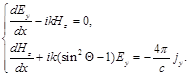   (1)

k = ω/c – wave number, с – speed of light, j – electric current density.

We have reflections coefficient R, transmission coefficient T and absorption coefficient A of thin metal film, when H-wave falling on this film [11]:

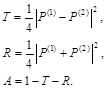(2)

Expression (2) contains P⁽¹⁾ and P⁽²⁾ [12] :

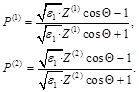(3)

Z⁽¹⁾ and Z⁽²⁾correspond to the impedance of lower surface the layer. In particular Z⁽¹⁾corresponds antisymmetric, in electric field, configuration of the external field: E_y(0) = -E_y(a), H_z(0) = H_z(a), and Z⁽²⁾ – corresponds symmetric configuration: E_y(0) = E_y(a), H_z(0) = -H_z(a) [11].

Expression for surface impedance in the case of interaction H-wave with the thin metal film, were obtained in [11] in the case when wavelength much more thickness of the thin layer:

(4)

For σ_a expression (this is electrical conductivity of the thin metal layer, with average thickness of this layer) we used results [13]. In this article we compared our results with experiment data [14]. Our σ_a expression have look:

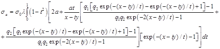(5)

x = a/(v_Fτ) – the dimensionless frequency of bulk electron collision, y = aω/v_F – the dimensionless frequency of the electric field, λ = x/(x-iy), σ₀ =ω²_pτ/4π  – the static electrical conductivity, v_F  – Fermi speed, τ – electron relaxation time, ω_p – plasma frequency, q₁ и q₂ – reflection coefficients.

Finally, reflection coefficient R, transmission coefficient T and absorption coefficient A (expression (2)) will have look [12]:

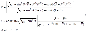(6)

ε_1,2 =ε₂/ε₁, .

Now we will begin to analyze behavior of this coefficients (expression (6)).

3. Results and Discussion

Let us consider behavior of coefficients R, T and A in the case of their frequency dependence with variation dielectric permeability value of the second environment ε₂ and in the case of different reflection coefficients q₁ and q₂. Clarify some parameters of potassium for further calculations: ω_p = 6.5 10¹⁵1/s, v_F  = 8.52 ∙ 10⁵ m/s, τ = 1.54 ∙ 10^-13 s, a = 10 nm.

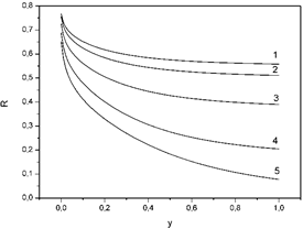
Figure 1. The dependence of reflection coefficients R on the dimensionless frequency of the electric field y. Curve 1: x = 0.002, θ = 20⁰, ε₁ = 1, ε₂ = 40, q₁ = 0.5, q₂ = 0.6; curve 2: x = 0.002, θ = 20⁰, ε₁ = 1, ε₂ = 30, q₁ = 0.5, q₂ = 0.6; curve 3: x = 0.002, θ = 20⁰, ε₁ = 1, ε₂ = 15, q₁ = 0.5, q₂ = 0.6; curve 4: x = 0.002, θ = 20⁰, ε₁ = 1, ε₂ = 5, q₁ = 0.5, q₂ = 0.6; curve 5: x = 0.002, θ = 20⁰, ε₁ = 1, ε₂ = 1, q₁ = 0.5, q₂ = 0.6.

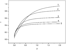
Figure 2. The dependence of transmission coefficients T on the dimensionless frequency of the electric field y. Curve 1: x = 0.002, θ = 20⁰, ε₁ = 1, ε₂ = 1, q₁ = 0.5, q₂ = 0.6; curve 2: x = 0.002, θ = 20⁰, ε₁ = 1, ε₂ = 5, q₁ = 0.5, q₂ = 0.6; curve 3: x = 0.002, θ = 20⁰, ε₁ = 1, ε₂ = 15, q₁ = 0.5, q₂ = 0.6; curve 4: x = 0.002, θ = 20⁰, ε₁ = 1, ε₂ = 30, q₁ = 0.5, q₂ = 0.6; curve 5: x = 0.002, θ = 20⁰, ε₁ = 1, ε₂ = 40, q₁ = 0.5, q₂ = 0.6.

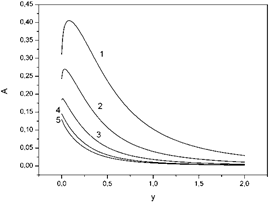
Figure 3. The dependence of absorption coefficients A on the dimensionless frequency of the electric field y. Curve 1: x = 0.002, θ = 20⁰, ε₁ = 1, ε₂ = 1, q₁ = 0.5, q₂ = 0.6; curve 2: x = 0.002, θ = 20⁰, ε₁ = 1, ε₂ = 5, q₁ = 0.5, q₂ = 0.6; curve 3: x = 0.002, θ = 20⁰, ε₁ = 1, ε₂ = 15, q₁ = 0.5, q₂ = 0.6; curve 4: x = 0.002, θ = 20⁰, ε₁ = 1, ε₂ = 30, q₁ = 0.5, q₂ = 0.6; curve 5: x = 0.002, θ = 20⁰, ε₁ = 1, ε₂ = 40, q₁ = 0.5, q₂ = 0.6.

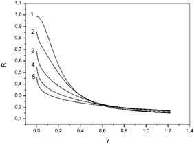
Figure 4. The dependence of reflection coefficients R on the dimensionless frequency of the electric field y. Curve 1: x = 0.002, θ = 20⁰, ε₁ = 1, ε₂ = 4, q₁ = 1, q₂ = 1; curve 2: x = 0.002, θ = 20⁰, ε₁ = 1, ε₂ = 4, q₁ = 0.8, q₂ = 0.9; curve 3: x = 0.002, θ = 20⁰, ε₁ = 1, ε₂ = 4, q₁ = 0.5, q₂ = 0.6; curve 4: x = 0.002, θ = 20⁰, ε₁ = 1, ε₂ = 4, q₁ = 0.2, q₂ = 0.3; curve 5: x = 0.002, θ = 20⁰, ε₁ = 1, ε₂ = 4, q₁ = 0, q₂ = 0.

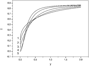
Figure 5. The dependence of transmission coefficients T on the dimensionless frequency of the electric field y. Curve 1: x = 0.002, θ = 20⁰, ε₁ = 1, ε₂ = 4, q₁ = 0, q₂ = 0; curve 2: x = 0.002, θ = 20⁰, ε₁ = 1, ε₂ = 4, q₁ = 0.2, q₂ = 0.3; curve 3: x = 0.002, θ = 20⁰, ε₁ = 1, ε₂ = 4, q₁ = 0.5, q₂ = 0.6; curve 4: x = 0.002, θ = 20⁰, ε₁ = 1, ε₂ = 4, q₁ = 0.8, q₂ = 0.9; curve 5: x = 0.002, θ = 20⁰, ε₁ = 1, ε₂ = 4, q₁ = 1, q₂ = 1.

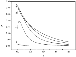
Figure 6. The dependence of absorption coefficients A on the dimensionless frequency of the electric field y. Curve1: x = 0.002, θ = 20⁰, ε₁ = 1, ε₂ = 4, q₁ = 0, q₂ = 0; curve 2: x = 0.002, θ = 20⁰, ε₁ = 1, ε₂ = 4, q₁ = 0.2, q₂ = 0.3; curve 3: x = 0.002, θ = 20⁰, ε₁ = 1, ε₂ = 4, q₁ = 0.5, q₂ = 0.6; curve 4: x = 0.002, θ = 20⁰, ε₁ = 1, ε₂ = 4, q₁ = 0.8, q₂ = 0.9; curve 5: x = 0.002, θ = 20⁰, ε₁ = 1, ε₂ = 4, q₁ = 1, q₂ = 1.

4. Conclusions

In figure 1 we can see that the descending velocity of the curve increases with increasing values of the dielectric permittivity of the second environment ε₂.

In figure 2 we can see that the increase velocity of the curve increases with increasing values of the dielectric permittivity of the second environment ε₂.

In figure 3, in the case of not large value of the dielectric permittivity (ε₂ < 30) we can see, that coefficient A increases, reaches maximum and descents. Cleary visible absorption maxima. In the case of large value of the dielectric permittivity (ε₂ > 30) coefficient A begin immediately descents.

In figure 4, 5, 6 we can see, that variation of the thin metal layer reflection coefficients q₁ and q₂ (from diffuse q₁ = q₂ = 0 to reflection q₁ = q₂ = 1 cases) affects to R, T, A coefficients. It is obvious that reflection coefficients will change, when the thin metal film borders with different environments. In particular, in figure 6, in the reflection case, coefficient A immediately descent. In all other cases coefficient A increases reaches its maximum and descents.

References

1. V.V. Kaminsky, N.N. Stepanov, M.M. Kazanin, A.A. Molodyh, S.M. Soloviev, Physics of the Solid State. 55 (5), 991 (2013)
2. K.L. Kliewer, R. Fuchs, Phys. Rev. 185 (3), 805 (1969)
3. F. Abeles, Optical properties of Metal Films. Physics of Thin Films, Ed. by M. H. Francombe and R. W. Hoffman (Academic, New York, 1971; Mir, Moscow, 1973)
4. W.E. Jones, K.L. Kliewer, R. Fuchs, Phys. Rev. 178 (3), 1201 (1969)
5. H. Kangarlou, M. Motallebi Aghgonbad, Optics and Spectroscopy. 115 (5), 753 (2013)
6. A.V. Latyshev, A.A. Yushkanov, Optics and Spectroscopy. 114 (3), 444 (2013)
7. T. Brandt, M. Hövel, B. Gompf, M. Dressel, Phys. Rev. B. 78 (20), 205409 (2008)
8. E.V. Zavitaev, O.V. Rusakov, A.A. Yushkanov, Physics of the Solid State. 54 (6), 1041 (2012)
9. A.V. Babich, V.V. Pogosov, Physics of the Solid State. 55 (1), 177 (2013)
10. A.N. Kondratenko, Penetration of waves in plasma. (Atomizdat, Moscow, 1979)
11. A.V. Latyshev, A.A. Yushkanov, Microelectronics. 41 (1), 27 (2012)
12. A.V. Latyshev, A.A. Yushkanov, Optics and Spectroscopy. 12 (1), 38 (2012)
13. A.I. Utkin , A.A. Yushkanov, Universal Journal of Applied Mathematics. 1 (2), 127 (2013)
14. Sun Tik, Yao Bo, Warren Andrew P., Kumar Vineet, Roberts Scott, Barmak Katayun, Coffey Kevin R, J. Vac. Sci. Technol. A. 26 (4) 605 (2008)