
International Journal of Mathematics and Computational Science, Vol. 1, No. 1, February 2015 Publish Date: Jan. 26, 2015 Pages: 1-4
Modeling Asphalt Concrete Mix Design Using Least Square Optimization
Saad Issa Sarsam*
Department of Civil Engineering, College of Engineering, University of Baghdad, Baghdad, Iraq
Abstract
This paper presents a computerized method for asphalt concrete job-mix formula design; the preparation of overall gradation of aggregates for mix design is considered as an essential step in the design of asphalt concrete mixture. The target gradation should be dense, uniform, and should not go for one extreme boundary to another or move along one of the boundaries. On the other hand, the maximum size of aggregates (start point of the gradation curve) and the percent filler (end of the gradation curve) are fixed for each type of asphalt concrete mix. The parabola fit using least square method was adopted in this paper; it cares for job mix formula mathematical equation smoothing. The developed program uses parabola fit method to find all possible equations that combines the various material gradations as per the specification requirements, the optimization process will select and print the best six formulas (eq. 1 to eq.6) ascended according to the sum of errors squares. Decision can be made by the user, and given to the computer to choose one of the six equations after considering the economic issue. For several months with every day execution of the program, it proved that it is efficient and quick enough to be used in such mix design.
Keywords
Asphalt Concrete, Design, Job-Mix Formula, Least Square, Optimization
Received: December 15, 2014
Accepted: December 31, 2014
Published online: January 23, 2015
@ 2015 The Authors. Published by American Institute of Science. This Open Access article is under the CC BY-NC license. http://creativecommons.org/licenses/by-nc/4.0/
1. Introduction
The asphalt concrete mix for base, binder and wearing courses, is composed basically of aggregate, coarse, medium, and fine in sizes, mineral filler and asphalt cement. The several mineral constituents are to be sized, uniformly graded and combined in such proportions that the resulting blend (job mix formula) meets the grading requirements for the specific layer type under contract. Such combinations are considered as 100% by weight of total aggregate in the mix. A study presented by [1] describes the application of general curve fitting procedure for AASHO Road test, which can be used for linear or non-linear models (least square residuals and minimum absolute residuals). He presented results that are obtained when the test data are summarized with models that are simpler in form and more comprehensive using a computer program than those employed in previous test report calculated by traditional methods. Another work by [2] studied the possibility of implementing the stepwise optimization in the design of asphalt concrete mix; he concluded that it is suitable for such purpose with accepted accuracy. On the other hand, [3] investigated the possibility of using the Mathematical Modeling technique in combining the aggregates of different sizes to meet the specification requirements; he concluded that Modeling the aggregate combination is efficient and quick for application in the mix design.
[4] Implemented computerized optimization for aggregate gradation, various mathematical expressions have been tried for such purpose, finally it was concluded that the Modeling phenomena is recommended replacing the current trial and error process usually adopted.
[5] Presented the specification requirements for various asphalt concrete layers and stated that the job mix formula should not vary from the lower limit of the specification requirements on the sieve to the higher limit on the adjacent sieve but should be uniformly- graded. Usually a dense gradation formula is employed in executing pavement of asphalt concrete type as illustrated in tables 1.
Asphalt concrete mix design equation is usually found manually using trial and error method. Although good results may be obtained, but it is certainly not the best and also consumes time. Difficulties appear using computer are the high process time for finding the optimum solution and the decision factors affecting the optimality sum of which are logical. The asphalt concrete is designed to produce a stable material of maximum durability and minimum cost. Such requirements are specified in terms of a target grading and permitted range of asphalt content, stiffness and voids. Various sizes of aggregates (coarse, medium, fine, sand, and filler) are combined theoretically using trial and error method to get the final gradation (job mix formula) which must satisfy the specification requirements. It was felt that using a computer program in such analysis may give more accurate and fast results. [6] Studied the setting up of a mathematical model to combine the aggregates in order to meet a desired grading. The process used is a linear programming technique. He concluded that optimum cost mixes can be achieved by using the obtained model to select and combine aggregates, filler and bitumen.
2. Methodology of Job Mix Formula Design
All of the gradation specification requirements for base, binder or wearing courses were stored in a file. The program first asks about the kind of specification to follow, then it gets it out from the file and tries to find an optimum job-mix formula according to specific objective function and certain constrains. The objective function is to find the smoothest curve inside the specification, while constrains are:
a.) The formula curve should be inside the specification area.
b.) The formula curve should be away from both extremes of the specifications (i.e. in the middle of the specification area if possible) so that the largest range of tolerance could be obtained.
c.) Logical constrains from economical point of view, satisfying all about objective function and constrains, may give a job mix formula that is not economical, for example it require high percentages of filler material.
Table 1. SCRB (2004) specification requirements for asphalt concrete
| Sieve size (mm) | Percent finer by weight | ||||
| Base course A | Base course B | Base course C | Binder course | Wearing course | |
| 37.5 | 100-90 | 100 | 100 | 100 | 100 |
| 25 | 95-77 | 100-87 | 100 | 100 | 100 |
| 19 | 90-68 | 95-80 | 100-92 | 100-88 | 100 |
| 12.5 | 83-55 | 90-70 | 95-82 | 87-65 | 95-75 |
| 9.5 | 75-47 | 85-65 | 92-75 | 80-55 | 88-65 |
| 4.75 | 65-33 | 75-50 | 82-60 | 64-37 | 75-50 |
| 2.0 | 50-20 | 65-33 | 70-42 | 45-23 | 55-32 |
| 1.0 | --------- | --------- | --------- | 34-17 | 42-24 |
| 0.6 | --------- | --------- | --------- | 27-13 | 35-18 |
| 0.425 | 30-10 | 40-17 | 45-20 | ------- | ------ |
| 0.250 | -------- | ---------- | --------- | 20-8 | 25-10 |
| 0.180 | 22-5 | 25-10 | 28-10 | ------- | ------- |
| 0.125 | --------- | ---------- | --------- | 15-6 | 20-8 |
| 0.075 | 10-3 | 10-3 | 10-3 | 10-5 | 12-6 |
3. Mathematical Derivation of Job Mix Formula
Least square optimization method were used to get the optimum objective function, the possible combination of points inside the specification are used to construct the mix gradation formula, then sum of squares errors of these points from calculated mathematical function like second order equation is calculated. Then the combinations of all sums of square errors of all possible combinations are executed to get the best formula. The mathematical function is derived from each combination of points using least square fitting. The job mix formula is assumed as:
Y = A0 + A1X + A2X2 (1)
Where X, Y, are the possible combination points, A0, A1, A2 are constrains derived using least square fitting method.
Y = % passing each sieve; X = size (mm).
The constrains are calculated using equations 2, 3, and 4 as follows:
![]() (2)
(2)
![]() (3)
(3)
![]() (4)
(4)
Where: w0 = Ʃ Yi; w1 = Ʃ Yi Xi; w2 = Ʃ Yi Xi2; w3 = Ʃ Yi Xi3; w4 = Ʃ Yi Xi4;
![]() ;
; ![]() ; v2 = Ʃ Xi;v3 = Ʃ Xi2;
; v2 = Ʃ Xi;v3 = Ʃ Xi2;
v4 = Ʃ Xi3; n = no. of points
After finding the function y = f(x) from (n) points (x1, y1) ……. (x n, y n) [note that X i represents particle size (mm) and Y represents percentage passing], summation of error squares is calculated using equation5 and 6.
![]() (5)
(5)
![]() (6)
(6)
A0, A1, A2, ERRK and all points (x1, y1) ……. (x n, y n) are kept for later stage in the program. Again, the program follows all above calculations but for new set of points to find also another smooth function with a new value of ERRK. The program always maintains all information (i.e. A0, A1, A2, ERRK and its points about the smoothest six formulas (formulas with least values of ERRK).
As shown in figure 1, all six-gradation formulas points with mixing values are printed and plotted. Equation 1 represents the formula with minimum ERRK, which means the best-derived formulas; equation 2 formula has largest ERRK and so on.
To satisfy the third constrain given in this paper, which is a logical constrain, one can choose any one of the six formula, for example equation 6 with 7% filler because equation 1 formula assumes 9% filler, which is not economical. From the graph in figure 1 it is obvious that there is no big difference in smoothing between equation 1 curve and equation 6 curve.
Table 2 shows the grain size distribution for each of the six equations selected by the least square optimization procedure and exhibited as an output. On the other hand, Table 3 demonstrates the percentages of each type of mineral aggregates required for each equation as supplied by the software.
Table 2. Grain size distribution output for each equation
| Sieve size (mm) | Percent finer by weight | |||||
| Equation 1 | Equation 2 | Equation 3 | Equation 4 | Equation 5 | Equation 6 | |
| 25 | 90.0 | 90.0 | 90.0 | 92.5 | 92.5 | 92.5 |
| 19 | 82.3 | 82.3 | 82.3 | 84.47 | 84.47 | 94.47 |
| 12.5 | 76.14 | 76.14 | 76.14 | 77.06 | 77.06 | 77.06 |
| 9.5 | 70.07 | 70.07 | 70.07 | 70.11 | 70.11 | 70.11 |
| 4.75 | 56.39 | 56.38 | 56.37 | 56.39 | 56.38 | 56.37 |
| 2.0 | 44.45 | 44.30 | 44.15 | 44.45 | 44.30 | 44.15 |
| 0.425 | 24.62 | 23.99 | 23.36 | 24.62 | 23.99 | 23.36 |
| 0.18 | 14.00 | 13.12 | 12.25 | 14.00 | 13.12 | 12.25 |
| 0.075 | 9.35 | 8.55 | 7.74 | 9.35 | 8.55 | 7.74 |
Table 3. Type and percentage of materials required for each equation
| % of material | Equation 1 | Equation 2 | Equation 3 | Equation 4 | Equation 5 | Equation 6 |
| Coarse aggregate | 20 | 20 | 20 | 15 | 15 | 15 |
| Medium aggregate | 5.0 | 5.0 | 5.0 | 10 | 10 | 10 |
| Fine aggregate | 25 | 25 | 25 | 25 | 25 | 25 |
| Sand | 41 | 42 | 43 | 41 | 42 | 43 |
| Mineral Filler | 9.0 | 8.0 | 7.0 | 9.0 | 8.0 | 7.0 |
Figure 2 illustrates the final setup of the selected equations and the design gradation. It shows that the tolerance of the J.M.F. is sited inside and within the specification requirements. On the other hand, Table 4 demonstrates the final output of the software, the gradation of asphalt concrete constituent materials are presented; the percentages of each type of aggregate, which provide the optimized job mix formula, are also shown.
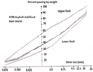
Fig. 1. Best six job mix formulas using Least Square Optimization method.
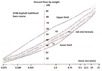
Fig. 2. Final Job mix formula design for Asphalt concrete Base course
Table 4. Final output showing the optimized job mix formula
| Sieve size (mm) | Percent finer by weight | |||||||||
| Mineral Aggregates Material types | Optimized Formula | J.M.F. Tolerance | Specifications | |||||||
| Coarse | Medium | Fine | Sand | Filler | J. M. F. | Upper | Lower | Max. | Min | |
| 37.5 | 100 | 100 | 100 | 100 | 100 | 100 | 100 | 100 | 100 | 100 |
| 25 | 50.2 | 100 | 100 | 100 | 100 | 90.0 | 87.0 | 96.0 | 87.0 | 100 |
| 19 | 20.5 | 64.0 | 100 | 100 | 100 | 82.3 | 80.0 | 88.3 | 80.0 | 95.0 |
| 12.5 | 0.9 | 19.2 | 100 | 100 | 100 | 76.1 | 70.1 | 82.1 | 70.0 | 90.0 |
| 9.5 | 0.0 | 0.8 | 80.1 | 100 | 100 | 70.1 | 65.0 | 76.1 | 65.0 | 85.0 |
| 4.75 | 0.0 | 0.0 | 27.2 | 99.0 | 100 | 56.4 | 50.4 | 62.4 | 50.0 | 75.0 |
| 2.0 | 0.0 | 0.0 | 2.4 | 85.0 | 100 | 44.2 | 40.2 | 48.2 | 33.0 | 65.0 |
| 0.420 | 0.0 | 0.0 | 1.0 | 37.0 | 100 | 23.4 | 19.4 | 27.4 | 17.0 | 40.0 |
| 0.180 | 0.0 | 0.0 | 0.2 | 12.2 | 100 | 12.2 | 10.0 | 16.2 | 10.0 | 25.0 |
| 0.075 | 0.0 | 0.0 | 0.2 | 4.2 | 84.8 | 7.7 | 6.2 | 9.2 | 3.0 | 10.0 |
| Percentages | 20.0 | 5.0 | 25.0 | 43.0 | 7.0 | |||||
4. Conclusions
Based on the limited investigation, the following conclusions may be drawn:
1. The least square optimization method for asphalt concrete mix design produces exactly the optimum objective function.
2. It provides the best six job mix formula after taking the specifications constrains into consideration.
3. It gives suggestion about the best job mix equation through optimization process, and allows the user to consider economic issues in deciding the final mix design equation.
4. The software output provides a summary of the tried equations and demonstrates the final optimized job mix formula with the required tolerance.
5. For several months and every day executing the program many times, it was proved that the least square optimization method is efficient and quick enough for five aggregate material sizes mixing, and is recommended to be used always.
References
- Irick P. (1963) "Application of general curve fitting procedure to AASHO road test data" HRB, Highway research record No. 42, USA.
- Sarsam S. (2013) "Stepwise Optimization Modeling of Asphalt Concrete Mix Design" Research Journal of Computation and Mathematics, RJCM 2013, 1(2): P (28-32); Sciknow Publications Ltd. USA.
- Sarsam S. (1997) "The design of asphaltic concrete mix using a mathematical model" Journal of Engineering and Technology Vol. 16 No. 3, University of technology, Baghdad, Iraq.
- Sarsam S. (2012) "Computerized Optimization of Asphalt Concrete Mix Design" Proceedings, International Conference on Management Sciences and Information Technology (MSIT 2012) Changsha, China, July 1-2, 2012
- SCRB (2004) "Standard specification for roads and bridges" Ministry of Housing and construction, Iraq
- Yeaman J. (1970) "The design of asphaltic concrete using mathematical models and linear programming techniques" Proceeding, ARRB – Vol.5 Part 5 Australia.


