
American Journal of Educational Science, Vol. 1, No. 4, September 2015 Publish Date: Jul. 10, 2015 Pages: 135-151
Systems Dynamics and Control, Proposed Course Overview and Education Oriented Approach for Mechatronics Engineering Curricula; Case Study
Farhan A. Salem1, 2, Ahmad A. Mahfouz2, 3, Ayman A. Aly1, 4, *
1Mechatronics Engineering, Dept. of Mechanical Eng., College of Engineering, Taif University, Taif, Saudi Arabia
2Dept. of Automatic and Mechatronics Systems, Vladimir State University, Vladimir, Russia
3Alpha Center for Engineering Studies and Technology Researches, Amman, Jordan
4Mechatronics Engineering, Dept. of Mechanical Engineering, Faculty of Engineering, Assuit University, Assiut, Egypt
Abstract
This paper extends writer's previous work, and applies proposed for Mechatronics engineering curricula, a ''system dynamics and control'' course education oriented methodology that integrates knowledge and abilities delivery, course topics, learning objective and outcomes. Methodology is intended to support educators in teaching process, help students in concepts understanding, maximum knowledge and skills gaining in solving controller/algorithm selection and design problems as a stage of Mechatronics system design stages, as well as, equip students with the key abilities and knowledge, required for further courses in mechatronics curricula.
Keywords
Mechatronics Education, Dynamics Control, Design, Modeling, Case Study
Received:May 27, 2015
Accepted: June 13, 2015
Published online: July 9, 2015
@ 2015 The Authors. Published by American Institute of Science. This Open Access article is under the CC BY-NC license. http://creativecommons.org/licenses/by-nc/4.0/
Contents
1. Introduction 2. Role of Control Subsystem in Mechatronics Design 3. Case Study: Applying Proposed Methodology; Single Joint (One DOF) Robot Arm Output Position Control 4. Solving Control Problem Applying Methodology Steps 4.1. Problem Statement 4.2. System Representation 4.3. Analysis and Evaluation of Basic Robotic Arm System 4.4. Selection and Design of Control System in Time Domain, to Meet and Maintain Desired Overall System Performance 4.5. Verification and Optimization 5. Conclusion
1. Introduction
The modern advances in information technology and decision making, as well as the synergetic integration of different fundamental engineering domains caused the engineering problems to get harder, broader, and deeper. Problems are multidisciplinary and require a multidisciplinary engineering systems approach to solve them, such modern multidisciplinary systems are called Mechatronics systems, correspondingly, engineers face daunting challenges, and to be competitive, in labor market, engineers must provide high value by being immediate, innovative, integrative, conceptual, and multidisciplinary, engineers must have depth in a specific engineering discipline, as well as multidisciplinary engineering breadth, with a balance between theory and practice, in addition, they must have breadth in business and human values, an engineer with such qualifications is called Mechatronics engineer. Mechatronics engineer is expected to design engineering systems with synergy and integration toward constrains like higher performance, speed, precision, efficiency, lower costs and functionality. [1] [2]
To fulfill Mechatronics engineering curricula requirements and meet such integrated abilities and knowledge requirements, In [2] is proposed, a ''system dynamics and control'' course simple but highly effective and tested education oriented teaching approach of knowledge and abilities delivery that integrates course topics, learning objective, outcomes in solving control system selection and design problems, and intended to support educators in teaching process, and help students in concepts understanding, maximum knowledge and skills gaining in solving controller/algorithm selection and design problems as a stage of Mechatronics system design stages, and to equip students with the key abilities and knowledge, required for further courses in mechatronics caricula including; Mechatronics fundamnetals, Mechatronics systems design, Process control, Embedded systems design, Robotics, PLC, CNC. This paper extends this work, the main concepts, topics CLOs and outcomes are discussed, and proposed selection and design steps (shown in Figure 1) are applied. The proposed education oriented teaching approach is supported by simple and easy to memorize education oriented design steps ,Tables (1:8) and graphs, that are recommended to provide students with, and ask to bring on every lecture, these are to help in integrating course CLOs, evaluating concepts and gaining integrated abilities and knowledge desired for further courses, where: In Table 1, the proposed course description and topics is explained in details, in particular, main topics mapped with their specific subtitles, objectives, number of lectures and weeks. In Table 2: Some basic rules of block diagram algebra. In Table 3; I and II order systems modeling, response measures, dominant pole approximation and general forms of transfer function. In Table 4 (a): Stable response forms and characteristics depending on damping ratio undamped natural frequency, poles location. In Table 4 (b) the nature of second order system poles (roots) and the effect of changing damping ratio and undamped natural frequency on systems response. In Table 5: the steady state error dependence on input signal and system type. In table 6: Control systems/algorithms transfer function, actions, selection criteria and root locus sketching rules. In table 7: state space representation and controller design. In table 8: Frequency domain performance measures, Nyquist and bode stability criterions and plots, controller design in frequency response
2. Role of Control Subsystem in Mechatronics Design
There are many definitions of Mechatronics, it can be defined as multidisciplinary concept, it is synergistic integration of mechanical engineering, electric engineering, electronic systems, information technology, intelligent control system, and computer hardware and software to manage complexity, uncertainty, and communication through the design and manufacture of products and processes from the very start of the design process, thus enabling complex decision making. Modern products are considered Mechatronics products, since, it is comprehensive mechanical systems with fully integrated electronics, intelligent control system and information technology. Such multidisciplinary and complex products, considering the top two drivers in industry today for improving development processes, that are shorter product-development schedules and increased customer demand for better performing products, demand another approach for efficient development. The Mechatronic system design process addresses these challenges, it is a modern interdisciplinary design procedure, it is the concurrent selection, evaluation, synergetic integration, and optimization of the whole system and all its sub-systems and components as a whole and concurrently, all the design disciplines work in parallel and collaboratively throughout the design and development process to produce an overall optimal design鈥no after-thought add-ons allowed, this approach offers less constrains and shortened development, also allows the design engineers to provide feedback to each other about how their part of design is effect by others. [1-2]
Mechatronics system is considered consisting of the following main integrated subsystems; mechanical subsystem, actuators subsystem, sensor subsystem, control unit subsystem, control algorithm subsystem and interfacing/conditioning. Mechatronics systems are supposed to be designed with synergy and integration toward constrains like higher performance, speed, precision, efficiency, lower costs and functionality and operate with exceptional high levels of accuracy and speed despite adverse effects of system nonlinearities, uncertainties and disturbances, Therefore, one of important decisions in Mechatronics system design process are, two directly related to each other subsystems, the control unit (physical-unit) and control algorithm subsystems selection, design and integration. Possible physical-control subsystem and algorithm options are shown in Figure 2. During the cuncurrent design of Mechatronic systems, it is important that changes in the mechanical structure and other subsystems be evaluated simultaneously; a badly designed mechanical system will never be able to give a good performance by adding a sophisticated control system, therefore, Mechatronic systems design requires that a mechanical system, dynamics and its control system structure be designed as an integrated system (this desired that (sub-)models be reusable), modeled and simulated to obtain unified model of both, that will simplify the analysis and prediction of whole system effects, performance, and generally to achieve a better performance, a more flexible system, or just reduce the cost of the system [1-2].
At control level during Mechatronics system design, three components can be identified; the control (physical control) unit, control algorithm and the electronic unit subsystems.The control unit is the central and most important part (brain) of Mechatronic system,it commands, controls and optimizes the process, by reading the input signals representing the state of the system and environment, compares them to the desired states, and according to control algorithm, outputs signals to the actuators to control and optimise the physical system and meeting specifications. Control subsystem must ensure excellent steady-state and dynamic performance [1-2]. The physical-controller subsystem, can be structured, Figure 1(b) Flowchart; design steps, for selection and design of control systems basically, around six basic forms (options) of programmable control system: Personal computer (PC), Microcomputer, Microcontroller (Mc), Digital signal processors (DSP), Application specific integrated circuits (ASICs) and Programmable logic controller (PLC) [1]. also, there are a variety of control algorithms exits, including: ON-OFF, PID modes, feedforward, adaptive, intelligent (Fuzzy logic, Neural network, Expert Systems and Genetic) control algorithms. The key factors that might influence the decision on selecting certain control unit/algorithm include; a) Operation (how system will run and how tasks/ instructions are processed), b) Robustness/environment (e.g. industrial, soft.), c) Serviceability (availability of replacement components and ease of repair/ replacement over controller life), d) Security (e.g. viruses), e) programming: Both programming environment (how control executes program) and language (e.g. C++) affect machine development time and operation f) unit cost, cost of final product, precision, required time to market, g) size-space saving, h) integration, i) processing power, also, safety criticality of the application, and number of products to be produced [3].
The ''system dynamics and control'' course, as basic course in control is structures around control algorithms selection and design, in particular, PID modes, and compensators Lead, lag, lead/lag, and their corresponding analogue control unit built based on amplifier, resistor/capacitors circuits, as well as, programming others units with these algorithms.
3. Case Study: Applying Proposed Methodology; Single Joint (One DOF) Robot Arm Output Position Control
This control problem is to be solved; applying proposed in [2], methodology and following proposed steps and flowchart shown in Figure 1 (a), (b), students can apply these steps in solving their course project control problems.
It is required to select and design a control system (algorithm) to control the output angular displacement of a pick and place robot arm, designed to pick an object from one location and place it on another location (angle range of 0o to 180o) corresponding to input voltage ,Vin (range of 0 to 12 Volts) .The designed control system is to ensure meeting and maintaining the following performance specification; settling time ,Ts=4s, OS% less than 1% and steady state error less than 0.1 of desired output
The robot arm system has the following nominal values; arm mass, M1= 8 Kg, arm length, L=0.4 m, arm width W= 0.05 m, viscous damping constant, bLoad = JLoad = 1, N. sec/m, end-effecter mass M2=0.2 Kg, of cuboid shape with b=h=0.05 m. The electric machine (actuator) has the following nominal values motor: Vin=12 Volts; Motor torque constant, Kt = 1.1882 Nm/A; Armature Resistance, Ra = 0.1557 Ohms (Ω); Armature Inductance, La = 0.82 MH; Geared-Motor Inertia: Jm = 0.271 kg. m2, Geared-Motor Viscous damping bm = 0.271 Nms; Motor back EMF constant, Kb = 1.185 rad/s/V, gear ratio, for simplicity, n=1, 0.01.
4. Solving Control Problem Applying Methodology Steps
4.1. Problem Statement
Before attempting to find a design solution for a given a problem, it is very important understanding what the problem and to state it in clear terms, this is half the solution [1]. the problem statement it is the process of gathering as much information as possible about: control problem objectives, the plant to be controlled, its purpose, structure, working principle, desired performance to meet and maintain, parameters... the problem statement include the following:
4.1.1. Control Objective
It is desired to select and design a control system (algorithm) to control the output angular position of single joint (1 DOF) pick and place robot arm, in reference to input voltage; that is to move the robot arm to the desired output angular position (angle range of 0 to 180), θL, corresponding to the applied input voltage, Vin (voltage range of 0 to 12).
4.1.2. Desired Performance Specification to Meet and Maintain
The designed control system is to ensure meeting and maintaining the following time domain performance specification; settling time, TS= 4s, OS% < 1% and Ess < 0.1 of desired output.
4.1.3. Variables to be Controlled
It is desired to move the robot arm to the desired output angular position θL , with angular displacement range of [0 to 180], corresponding to the applied input voltage, Vin with range of [0 to 12].
Input = Voltage, Vin, output =angular displacement of robot arm, θL.
Notice that the input variable could be the desired output arm angular displacement (that can be converted to corresponding voltage, or the actuator armature current required to move the load)
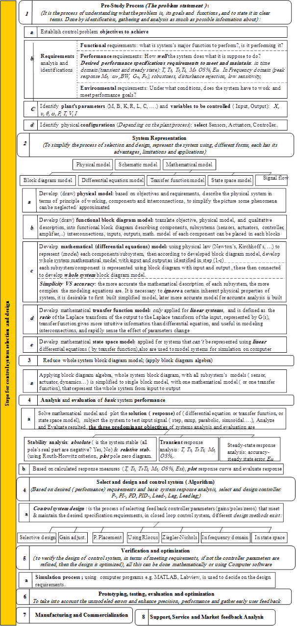
Figure 1 (a). proposed design steps, for selection and design of control systems.
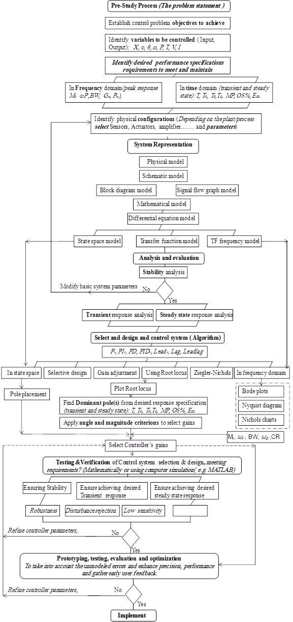
Figure 1 (b). Proposed flow chart, for selection and design of control systems.
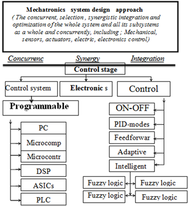
Figure 2 (a). Components at control stage; Control system/ algorithm electronic unit subsystems.
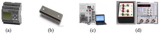
Figure 2 (b). (physical) control systems options, a) PLC, b) Microcontroller, c) Computer control, d) analog controllers.
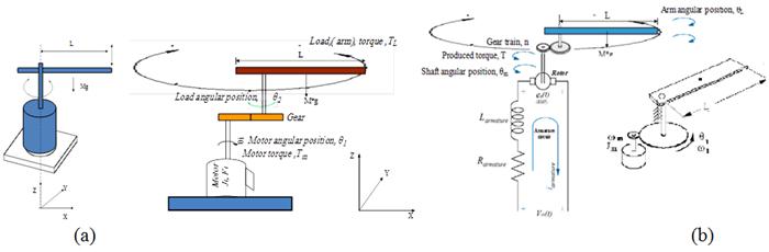
Figure 3. (a)(b) Schematic model of the plant; a single joint (one DOF) pick and place robot arm driven by an armature-controlled DC motor.
4.1.4. Physical Configurations
The pick and place robot system (plant) consists of three main physical parts (subsystems); arm-end-effecter with their dynamics, connected to actuator (for motion generation) through gear train with gear ratio, n, sensor for measuring output angular displacement. A suitable, available and easy to control actuator and sensor are PMDC motor and potentiometer. A simplified plant configuration (without control system components) is shown in Figure 3 (a) (b),
4.1.5. Plants Parameters
DC motor sizing; the DC motor is to be selected to generate required torque, operating with input 12 volts; to move the load to desired position with suitable speed. Parameters to consider are arm system nominal values; M, L, W, B, J, a, b and the PMDC parameters: L, R, Kt, Kb, Bm.
4.2. System Representation
System can be represemt in different ways, including; block diagram model, differential equation model, transfer function model, state space equations model, as well as physical and schematic models.
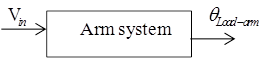
4.2.1. Plant Block Diagram Model (Basic System)
Based on arm system identified configurations, and schematic model shown in Figure 4 (a), the block diagram model shown in Figure 4 (b) is developed. Where based on the input voltage, the actuator (DC motor) generates angular motion, which will be reduced by gear train and transmitted to the arm, which will turn to corresponding angle. This series block connections can be reduced to single block of the whole arm (plant) system relating input voltage and arm output angular position.
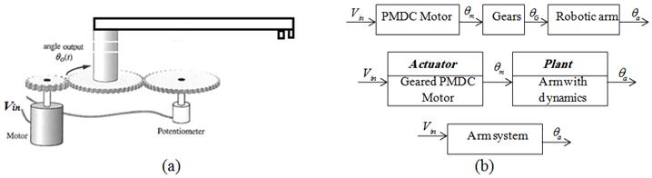
Figure 4. (a) Schematic and (b) Block diagram model of basic arm system.
4.2.2. Mathematical Modelling
Mathematical modelling is the process of representing a system using mathematical equations or logic. Based on basic system's (plant's) identified configurations and block diagram representation shown in Figure 4; each plant's component, in particular, PMDC motor, Gear train, and arm with dynamics, is to be represented mathematically, then an overall plants mathematical model is to be developed by joining these separate models in one whole arm model.
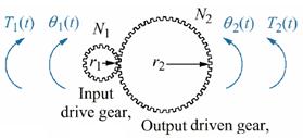
Figure 5. Interaction between two gears [4].
(i) Mathematical model in the form of differential equation:
(ii) Gear train modelling: Gears are used to obtain more speed and less torque or less speed and more torque. The interaction between two gears is depicted in the Figure 5, and modelled by gear ratio, n, given by Eq. (1) [4]
![]() (1)
(1)
(iii) Modelling the PMDC motor actuator
The electric machine-actuator most used in mechatronics systems design (including robotic arms), is PMDC motor. PMDC is an example of electromechanical systems with electrical and mechanical componentsa simplified equivalent representation of PMDC motor's two components are shown in Figure 6, Based on Newton's laws combined with the Kirchoff's laws, the mathematical model of PMDC motor in the form of differential equations describing electric and mechanical characteristics of the motor, and relating input volatge and output angiular displacement, can be derived [4],
(iv) Modelling motor's electrical characteristics
The coils of PMDC motor are consider as simple series (R-C circuit) inductor, resistor, with back EMF voltage, all subjected to input voltage, where applying a voltage to PMDC motor coils produce a torque in the armature. The torque developed by the motor, Tm,is related to the armature current, ia, by a torque constant Kt, and given by Eq.(2):
Motor Torque = Tm = Kt* ia(2)
The back electromotive force, EMF voltage, ea is induced by the rotation of the armature windings in the fixed magnetic field, and given by Eq. (3):
![]() (3)
(3)
Applying Kirchoff's law around the electrical loop by summing voltages throughout the R-L circuit gives Eq. (4):
![]() (4)
(4)
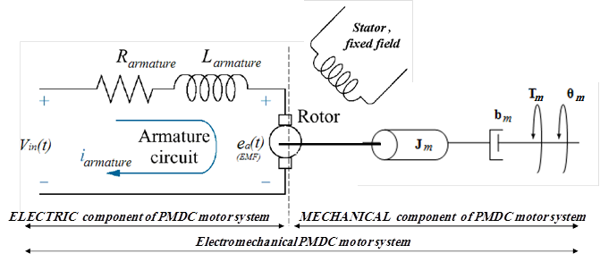
Figure 6. A simplified equivalent representation of the PMDC motor's electromechanical components [4].
Applying Ohm's law, substituting, taking Laplace transform and rearranging, we get differential equation that describes the electrical characteristics of PMDC motor, as given by Eq. (5, 6):
![]()
![]() (5)
(5)
Vin(s) = RaI(s) + Las I(s) + Kbs θ(s)
(Las +Ra) I(s) = Vin(s) - Kb sθ(s)(6)
(v) Modeling motor's Mechanical characteristics
The rotating shaft of PMDC motor is considered consiting of two mechanical rotaional components series Mass- Damper, under the input of generated motor torqe, where the torque, developed by motor, produces an angular velocity, ω= dθ/dt, according to the inertia, J and damping friction, b, of the motor and load. Performing the energy balance on the PMDC motor system; the sum of the torques must equal zero, gives Eq.(7):
![]()
Te - Tα -Tω - TEMF = 0(7)
Considering that system dynamics and disturbance torques depends on arm shape and dimensions, the mechanical DC motor part, will have the form given by Eq. (8):
Kt ia = Tα + Tω + Tload +Tf(8)
Where: Kt: torque constant, ia: armature current, Tload: load torque, Tα: torque due to acceleration= Jmd2θ/dt2, Tω torque due to velocity = bmdθ/dt,. The coulomb friction can be found at steady state by:
Kt ia - b*ω= Tf(9)
Substituting the following values: Te = Kt*ia, Tα = Jm*d2θ/dt2, and Tω= bm*dθ/dt, in open loop PMDC motor system without load attached, that is the change in Tmotor is zero, gives equation that describes the mechanical characteristics of PMDC motor, gives Eq. (10). Taking Laplace transform and rearranging gives Eq. (11):
![]() (10)
(10)
Kt*I(s) - Jm *s2θ(s)-bm*s θ(s) = 0
KtI (s) = (Jm s + bm) s θ(s) (11)
The electrical and mechanical PMDC motor two characteristics are coupled to each other through an algebraic torque equation given by Eq.(2).
(vi) Deriving PMDC motor open loop system transfer functions
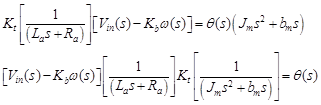
To derive the PMDC motor transfer function, we need to rearrange Eq. (6) describing electrical characteristics of PMDC, such that we have only armature current ,I (s) on the right side, then substitute this value of armature current, I (s) in Eq. (11) describing PMDC mechanical characteristics, as follows:
![]() (12)
(12)
The PMDC motor electric component transfer function relating input armature current, I (s) and voltage, is given by:
![]() (13)
(13)
The PMDC motor Mechanical component transfer function in term of output torque and input rotor speed is given by:
![]() (14)
(14)
In case, no load attached, Tload =0, we have:
![]()
Now, Substituting (12) in (11), gives:
![]() (15)
(15)
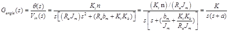
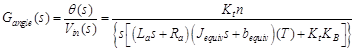
Rearranging (15), and knowing that the electrical and mechanical PMDC motor components are coupled to each other through an algebraic torque equationgiven by (2), we obtain the PMDC motor open loop transfer function without any load attached relating the input voltage, Vin(s), to the motor shaft output angle, θm(s), (or gear θG(s),) and given by Eq. (16):
![]() (16)
(16)
Dominant poles approximation: Eq. (16) is third order system, it can be approximated based on dominant poles. considering that the electric time constant is much smaller that the mechanical time constant, that is the armature inductance, La, is small compared to the armature resistance, Ra, which is usual for a DC motor), based on this, substituting La=0 in Eq. (16) will result in second order transfer function given by Eq. (17), we can also, Substitute defined PMDC motor parameters, and finding poles, selecting dominant poles will result in same results,
 (17)
(17)
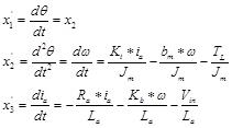
(vii) Mathematical modelling of PMDC motor in state space equations form:
The state variables (along with the input functions) used in equations describing the dynamics of a system, provide the future state of the system. Mathematically, the state of the system is described by a set of first-order differential equation in terms of state variables. The state space model takes the below form, rearranging Eqs.(5) and (10) to have the two first order equations given by (18) (19), relating the angular speed and armature current:
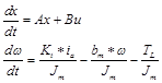 (18)
(18)
 (19)
(19)
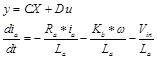
Taking the DC motor position θ, as the output, and choosing the state variable to be position θm, velocity ωm and armature currents ia, Substituting state variables, in electric and mechanical part equations and rearranging gives:

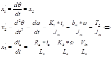
Substituting state variables and rearranging gives, the following state space model given by Eq. (20):
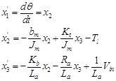
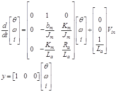 (20)
(20)
(viii) Arm dynamics modeling:
There are dynamic requirements, which have to be satisfied depending on the motion and trajectories, where if fast motions are needed, these dynamic effects may dominate static phenomena, [6-8]. To model, Simulate and analyze the open loop robot arm system, considering that the end-effecter is a part of robot arm, the total equivalent inertia, Jequiv and total equivalent damping, bequiv at the armature of the motor are given by Eq. (21). To compute the total inertia, Jequiv, robot arm is consider as thin rod of mass m, length ℓ, (so that m = ρ*ℓ*s), this rod is rotating around the axis which passes through its center and is perpendicular to the rod, end-effecter is assumed of cuboid shape, the rod is rotating around the axis which passes through its center and is perpendicular to the rod. The moment of inertia of the robot arm can be found by computing integral given by Eq. (22), The moment of inertia of the cuboid end-effecter can be found by Eq. (23). General torque required from the motor is the sum of the static and dynamic torques, assuming the robot arm is horizontal, that is, the weight is perpendicular to the robot arm, the motor required torque is given by Eq. (24), substituting arm and effecter inertias and manipulating, gives Eq. (25).
![]()
![]() (21)
(21)
![]() (22)
(22)
![]() (23)
(23)
![]() (24)
(24)
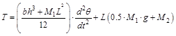 (25)
(25)
Now, based on derived mathematical models of basic plant (arm system) parts, and, Considering that system dynamics and disturbance torques depends on arm shape and dimensions, a unified mathematical model of arm system in the form of transfer function can be derived, that relates the input voltage with gears shaft (Load-arm) output angular displacement, and given by Eq. (26), where: T the disturbance torque, is all torques including coulomb friction
 (26)
(26)
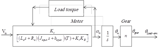
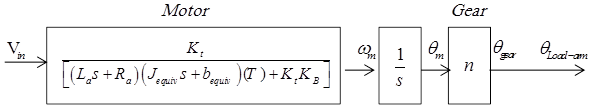
Based on derived mathematical model as shown in Eq. (27), the block diagram model of open loop basic plant (arm system) shown in Figure 7 (a), is derived, where the electrical and mechanical PMDC motor two characteristics are coupled to each other through an algebraic torque constant Kt, all motor can be simplified to get PMDC motor as one block, as shown in Figure 7 (b)
 (27)
(27)
(a)
(b)
(c)
Figure 7. (a) (b) (c) The block diagram model of open loop basic plant (arm system).
4.3. Analysis and Evaluation of Basic Robotic Arm System
Performance evaluate is accomplished by analysis of its performance including; stability analysis, transient and steady state response analysis, robustness, sensitivity and disturbance rejection.
Table 1. Calculated response specifications of original system.
| Measure | TR | TP | TS | T | OS%, | ESS | ζ | ωn |
| Original III order | 2.55 | - | 4.59 | 1.3 | 0 | 0 | - | - |
| App. II order | 2.63 | - | 4.68 | 1.2 | 0 | F | 4.6641 | 7.7078 |
| App. I order | 2.63 | - | 4.68 | 1.2 | 0 | F | - | - |
4.3.1. Stability Analysis
The derived plant transfer function is type one third order system; to analyze stability we first to consider arm dynamics including arm system damping and inertia parameters. The dampening and inertia components of the arm system are calculated by Eq. (28) and adjusted by the gear ratios, n. where bm= 0.271, Jm = 0.271, for now JLoad = JLoad = 1.
![]()
![]() (28)
(28)
For demonstration of system approximation and introducing dominant pole concept, two transfer function models are to be used, the approximated as second order given by Eq. (16),and the original third order system model given by Eq. (17). Substituting defined and calculated parameters values in both equations and finding closed loop transfer function, will result in Eq. (29) with three poles (-0.8413, -0.9391 ±9.2315i) and Eq. (30) approximated system with two poles (-71.0640, -0.8360), both systems are stable, since the roots real part is negative and located on the LHP, if the system is not stable then the arm system parameters (arm, DC motor, gear ratio ) are adjusted to result in stable system. More over in both cases we see that a single dominant pole exists that is -0.8360, based on this, the system can further be approximated as first order system given by Eq. (31). Plotting original III order and approximated as II order transfer functions, as well as approximated as I order, in the same graph window using MATLAB, will result in response curve shown in Figure 8 (a), the three response curves are almost identical.
Stability in state space: The problem of transforming a regular matrix into a singular matrix is referred to as the eigenvalue problem, the eigenvalues are equal to the poles, and given by: ![]()
4.3.2. Transient and Steady State Response Analysis
Applying expressions for calculating performance measures (for underdamped response case), including T, TR, TP, TS, MP, OS%, ESS by expressions given by Eqs (32), for the original and approximated systems, as well as, from MATLAB step response characteritics, will result in values, listed in table 1. Response anlysis of basic plant can be supported by plotting root locus for the original III order system bode and nyquist diargams, and with the help of Routh-Howrwits stability criterion. The root locus, Bode and Nyquist plots using MATLAB is shown in Figure 8 (b),(c).
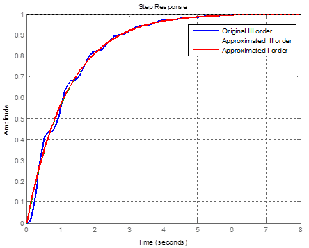
Figure 8 (a). Response curves of original and approximated arm (plant) system.
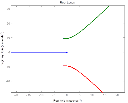
Figure 8 (b). The root locus plot using MATLAB of original III order system.
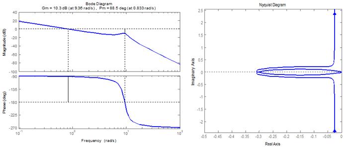
Figure 8 (c). Bode and Nyquist plots using MATLAB of original III order system.
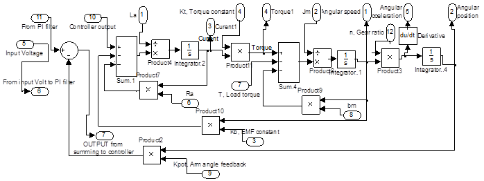
Figure 9 (a). DC machine subsystem model.
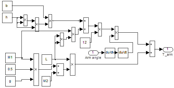
Figure 9 (b). Robot arm torque Simulink model.
4.3.3. Performance Evaluation
Based on calculated performance measures, Routh-Howrwits stability criterion analysis and other plots, it is found, the arm system in terms of output angular position, is third order, type one stable system, with overdamped slow response, (ζ =4.6641 and ωn =7.7078 rad/s), with settling time TS=4.59s, for unity step input, the system reaches steady state in 6.5 seconds. The system will be critically (marginally) stable for gain K= 3.2964, corresponding to gain margin of 10.3 dB and phase margin of 88.5 deg. Meanwhile desired performance are TS =4s, OS% less than 1% and Ess less than 0.1 of desired output. A control system is required to achieve and maintain the desired performance
Simulink can be used to develop simulation model of the arm system, shown in Figure 9, defining parameters and running models will result in response curve similar to those shown in Figure 8 (a), these response curves, are used to find transinet and steady state performance measures using MATLAB figure window tools.
![]() (29)
(29)
![]() (30)
(30)
![]() (31)
(31)
![]() (32)
(32)
4.4. Selection and Design of Control System in Time Domain, to Meet and Maintain Desired Overall System Performance
The term control system design refers to the process of selecting feedback gains that meet design specifications in a closed-loop control system. Most design methods are iterative, combining parameter selection with analysis, simulation, and insight into the dynamics of the plant [1]. Feedback (closed) loop configuration is most selected to control systems behaviour, consisting of control unit/algorithm, sensor and summing device, shown in Figure 10 (a) (b) (c), the input to the system is the desired output angle, that is converted to corresponding volt by input potentiometer, that in turn inputted to the system.
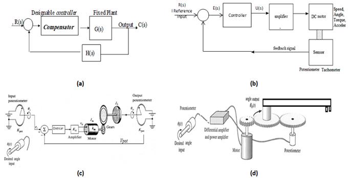
Figure 10. Feedback loop configuration.
4.4.1. Control Algorithm Selection
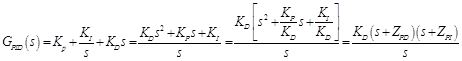
Control algorithms include P-, PI-, PD-, PID-, Lead, Lag, laglead. Since it is desired to inprove both transient and steady state responses, a suitable control system algorithm would be PID with transfer fuction model given by Eq. (33). The PD controller can also be selected, because it provides the ability to handle fast process load changes (e.g. in Pick and place robot), also PD controller reduces the amount of overshoot [9-11]. PID is equivalent to the adition of two zeros and one pole at origin.
![]() (33)
(33)
4.4.2. Sensor Modelling
To calculate the error, we need to convert the actual output robot arm position, into voltage, V, then compare this voltage with the input voltage Vin, the difference is the error signal in volts. Potentiometer is a popular sensor used to measure the actual output angualr position. Two potentiometers are used Input and output potentiometers. The user inputs the desired output maximum angle, then an input potentiometer converts it to corresponding input voltage to controller, the sensor- potentiometer converts the actual output arm angular displacemnet θL, into corresponding volt, Vp and then feeding back this value to controller that calcultes the error (Verror= Vin- Vp), the Potentiometer output is proportional to the actual robot arm position, θL.. the block diagram representation of the whole system with controller added (closed loop-feedback system), will have the form shown in Figure 11 (a)(b).
The output voltage of potentiometer is given by Eq.(34), where Kpot the potentiometer constant; It is equal to the ratio of the voltage change to the corresponding angle change. Depending on maximum desired output arm angle and maximum input voltage, the potentiometer can be chosen, for our case Vin= 0:12, and output angle = 0:180 degrees, substituting, we have potentiometer-sensor transfer function. Since the input and output potentiometers are configured in the same way, their transfer functions will be the same
![]() (34)
(34)
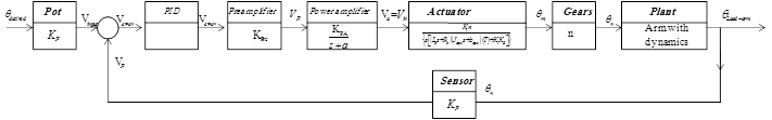
(a)
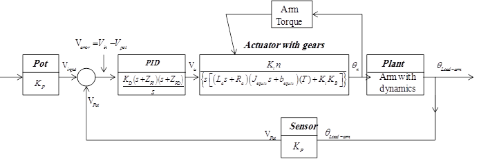
(b)
Figure 11. System block diagram.
4.4.3. Differential Preamplifier
As a part of feedback control system components differential preamplifier (voltage subtractor) is used. it is a type of electronic amplifier that amplifies the difference between two voltages, (difference between two potentiometers voltages). The preamplifier is used to determine the small voltages between to input voltages to calculate the error signal. The purpose of the preamplifier is to increase the power of a signal by the use of external source, that is to take the input signal voltage and output a voltage that the power amplifier can use. The transfer function of differential preamplifier is given as pure gain, and is given by Eq.(35). Power Amplifier: it takes the output voltage from the Preamplifier and converts it to a Voltage that is useable by the motor. This requires the Power Amplifier to output a significant amount of power, something that the Preamplifier is not capable of. The power amplifier transfer function is given by Eq. (36)
![]() (35)
(35)
![]() (36)
(36)
4.4.4. Control System Design
To design PID control (or any other) in time domain, we first, need to plot rool locus using the arm original III order open loop system transfer function, applying root locus skitching rules. Then from desired performance specifications (T, TS, OS%,) find damping ratio and undamped natural frequency, then find the dominant pole given by Eq.(37), finally applying angle and mgnitude criterion given by Eq. (38) to calculate the (added by controller) zeros/poles angles and gains of selected (e.g. PID) controller. Bode diagram can be used to design controller (e.g. lead, lag) in frequency domain.
![]() (37)
(37)
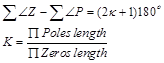 (38)
(38)
Before designing selected control algorithm; It is desired that OS% less than 1%, we consider the worst case it to be OS% = 0.1%, and by Eq. (39), or from plot of damping ratio against OS% shown in Figure 12 , we find the damping ratio to be ζ= 0.8261. Also It is desired that Ts=4s by Eq. (40), we find undamped natural frequency to be ωn= 1.2105 rad/s, based on this the dominant poles will be as given by Eq. (41), and the overall arm system with controller, sensor and all components can be approximated with as second order transfer function given by Eq. (42), such system when subjected to unit step response will have Ts =3.28 s and OS% = 1%, this response is shown in Figure 13 (a), to slow up response we can reduce undamped natural frequency to be ωn=1 rad/s; this will result in response curve shown in figure 13 (b) and the dominant pole will have the value P= -0.8261 + 0.5635i
![]() (39)
(39)
![]() (40)
(40)
![]() (41)
(41)
![]() (42)
(42)
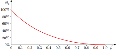
Figure 12. Relation between the damping ratio and OS%.
4.5. Verification and Optimization
To check if the desired performance specification (Ts=4s, OS% < 1% and Ess < 0.1) are achieved, if not the controller gains are refined and resulted performance checked again. To do this we need to find overall system closed loop transfer function and analyse the resulted response. The verification can be supported MATLAB-Simulink, where a Simulink model shown in Figure 14 is developed, and parameters of all components to be defined in MATLAB, finally then tested. The designed controller transfer function is given by Eq.(44), the forward transfer function is given by Eq. (45), and the closed loop overall transfer function is given by Eq. (55), subjecting the closed loop overall system transfer function to step input of R(s)=12/s, will result in response curve shown in Figure 15(a), the designed controller require adjustment to meet desired response. Tuning controller parameters we find the PD zero at ZPD= 0.001999 and PI zero at ZPI=- 0.0001901with gain equals to 1800 to result in response curve shown in Figure15 (b). The controller can be tuned further to achieve desired output performance
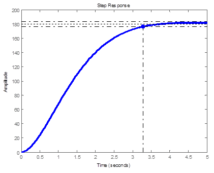
Figure 13 (a). Step response of approx. overall arm system with ζ= 0.8261 and ωn= 1.2105 rad/s.
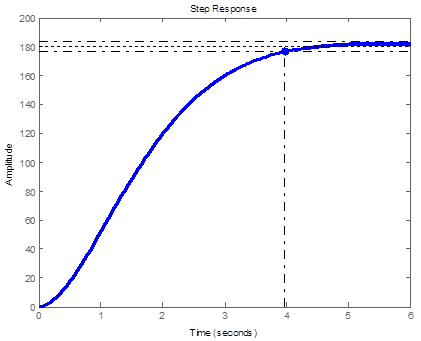
Figure 13 (b). Step response of approx. overall arm system with ζ= 0.8261 and ωn= 1 rad/s.
Designing selected control algorithm; this is acomplished by locating the dominant pole on root locus plot, then since PID controller is a combination of PD and PI controller given by Eq. (43), first we design a PD controller to achive transient response then designing PI controller to achieve steady state error.
PD controller is equivalent to addition of single zero to root locus, that is found applying angle criterion and the gain is found applying magnitude criterion. Also, PI is equivalent to the addition of pole at origin and zero that is found applying angle criterion.MATLAB siso tool can be used to design control system, with built in funtion, sisotool (). Designing we find the PD zero at ZPD= -0.001345 and PI zero at ZPI=-0 .0001901 with gain equals to 1880.
 (43)
(43)
![]() (44)
(44)
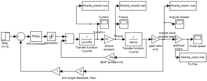
Figure 14. DC motor Simulink model with PID control.
![]() (45)
(45)
![]() (46)
(46)
5. Conclusion
Applying proposed for Mechatronics engineering curricula a ''system dynamics and control'' course education oriented methodology steps, flowcharts and tables, a case study of single joint robot arm output position control is introduced, the arm system is modelled, analysed, evaluated and a control system/algorithm are selected and designed to meet desired specifications.
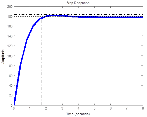
Figure 15 (a). Closed loop step response of arm system with PID controller.
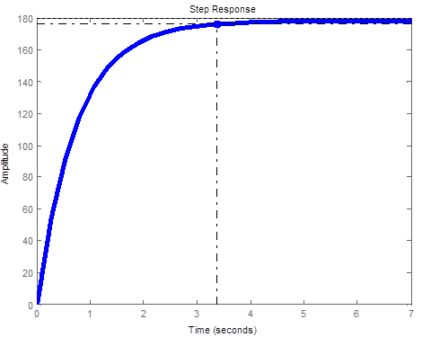
Figure 15 (b). Tuned closed loop step response of arm system with PID controller.
References
- Farhan A. Salem, Ahmad A. Mahfouz, Mechatronics Design And Implementation Education-Oriented Methodology; A Proposed Approach, Journal of Multidisciplinary Engineering Science and Technology (JMEST), Vol. 1 Issue 3, October, 2014.
- Farhan A. Salem, Ayman A. Aly, "PD Controller Structures: Comparison and Selection for an Electromechanical System", PP.1-12, Vol. 7, No. 2, I. J. Intelligent Systems and Applications (IJISA) January 2015. Farhan A. Salem, The role of control system/algorithm subsystems in Mechatronics Systems Design.
- Norman S. Nise, ''Control Systems Engineering'', 4th edition, Wily and sons, 2008.
- Farhan, A. Salem, ''Mechatronics design, modelling, controller selection, design and simulation of a Robot arm; Research and Education (III)'', Vol. 5 Issue 5, p39, Apr2013.
- Selig J. M.: Geometrical Methods in Robotics. Wiley, 1985.
- Shimon Y. Nof: Handbook of Industrial Robotics. Wiley, 1985.
- Emese Sza, Deczky- Krdoss, Ba´ Lint kiss , design and control of a 2DOF positioning robot ,10th IEEE International Conference on Methods and Models in Automation and Robotics , 30 August - 2 September 2004, Miedzyzdroje, Poland.
- D. D. Siljak, Decenralized Control of Complex System, New York Academic, 1991.
- Farhan A. Salem, Controllers and Control Algorithms: Selection and Time Domain Design Techniques Applied in Mechatronics Systems Design (Review and Research), International Journal of Engineering Sciences, 2 (5), PP 160-190, May 2013.
- Ayman A. Aly, Farhan A. Salem,Design of Intelligent Position Control for Single Axis Robot Arm , International Journal of Scientific & Engineering Research, Volume 5, Issue 6, June-2014.
- Farhan A. Salem, Ayman A. Aly, Mosleh Al-Harthi and Nadjim Merabtine, "New Control Design Method for First Order and Approximated First Order Systems", International Journal of Control, Automation And Systems (IJCAS) V4 (2), PP 7-17, 2015.


