
American Journal of Educational Science, Vol. 1, No. 3, July 2015 Publish Date: Jun. 10, 2015 Pages: 60-68
Enhanced Confidence Based Q Routing for an Ad Hoc Network
Rahul Desai1, *, B. P. Patil2
1Research Scholar, Sinhgad College of Engineering, Army Institute of Technology, Pune, India
2Department of Electronics & Telecommunication, Army Institute of Technology, Pune, India
Abstract
Confidence-based Q (CQ) Routing Algorithm is an adaptive network routing algorithm. CQ Routing Algorithm uses confidence values to improve the quality of exploration over standard Q routing. The Enhanced confidence Based Q routing which uses Variable of Decay Constant and Update All Q value approaches for updating the C values of non-selected Q values. Thus as compared with standard CQ routing, enhanced Q routing takes less amount of time to represent real state of the network, thus quality of exploration is improved. The performance of ECQ and CQ Routing Algorithms are compared to prove this improvement. Also the ECQ routing is compared with some existing routing protocols to judge the quality of the network in terms of some performance parameters such as packet delivery ratio, delay, control overhead and throughput.
Keywords
Q Routing, Reinforcement, CQ Routing, CDRQ Routing, ECQ Routing
Received:April 27, 2015
Accepted: May 13, 2015
Published online: June 8, 2015
@ 2015 The Authors. Published by American Institute of Science. This Open Access article is under the CC BY-NC license. http://creativecommons.org/licenses/by-nc/4.0/
1. Introduction and Survey of Existing Routing Protocols Over an ad Hoc Network
Ad hoc networks are infrastructure less networks where each node is acting as a router and perform the functions of routing – taking decision whom to forward and forwarding packets to next hop node in order to reach the packet in shortest amount of time. All nodes are mobile nodes; they are free to move inside and outside of a network. There are two types of protocols – proactive routing protocols and on demand also known as reactive routing protocols are widely used for an ad hoc network. Proactive routing protocols always maintains routing tables inside cache or routing tables and thus whenever there is necessity to forward the packets, path is readily available in cache / tables. While on demand routing protocols obtain the paths only when required to transmit the packets to the destination.
Destination Sequence Distance Vector (DSDV) [1] is one of oldest protocol comes under the category of proactive routing protocols. It uses distance vector mechanism to obtain distances in order to reach to the destination. Every node in the network communicates the distances to the neighbor nodes and thus obtains the path to reach to the destination. It also uses sequence numbers to avoid count to infinity problem which is major concern in distance vector routing protocols.
Optimized Link State Routing protocol is also proactive routing protocol and based on link state algorithm. In this, every node propagates the link state information to all other nodes in a network. In order to optimize further, only Multipoint relay (MPR) are allowed to broadcast this information.
In on demand routing protocols, route to the destination is obtained only when there is a need. When source nodes want to transmit data packets to the destination nodes, it initiates route discovery process. Route request (RREQ) messages float over the network and finally the packet reaches to the destination, Destination nodes replies with route replay message (RREP) and unicast towards the source node. All nodes including the source node keeps this route information in caches for future purpose.
Dynamic Source Routing Protocol (DSR) [2,3] is thus characterized by the use of source routing. The data packets carry the source route in the packet header. When the link or node goes down, existing route is no longer available; source node again initiates route discovery process to find out the optimum route. Route Error packets and acknowledgement packets are also used.
Ad Hoc on Demand Distance Vector Routing (AODV) [4] is also on-demand routing protocol. It uses traditional routing tables, one entry per destination. In AODV, only one route path is available in routing table, if this path fails, it again initiates route discovery process to find out another optimum path.
2. Survey of Q Routing - Reinforcement Based Routing
There are some agents present in systems or environment which learn from the system and tries to improve the system by reward-penalty fashion [5]. Q routing is based on reinforcement learning, where each node contains Q table (Similar to routing tables) which contains approximate delays to reach to the destination when the packet is forwarded to the next hop [6]. Thus each node in the network contains reinforcement learning module which tries to find out the optimum path to the destination. As illustrated in Figure 1, Let QX(Y, D) represents the time that a node X takes to deliver a packet P to the destination node D when the packet is transmitted to the next neighbor node Y. After sending the packet, node X will also get node Y’s estimate of the remaining time in the network[7,8].
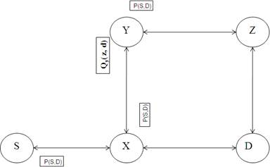
Figure 1. Reinforcement Learning.
Thus for every incoming packet, nodes consult its Q table and decides the next hop based on the least delivery time required to reach the packet to the destination. At the same time the sending node receives the estimate of the remaining delivery time for the packet to the destination. Thus after every packet transmitted by the source node and all intermediate nodes, Q values are received by these nodes and updates their Q table to represents the steady state of the network [7,8].
As soon as the node X sends a packet P to the destination node D to one of the neighboring nodes Y, node Y send back to node X, its best estimate QY(Z, D) for the destination D. QY(Z, D) for the destination D shows its remaining time required to reach the packet to the destination node D. Upon receiving QY(Z, D), node X computes the new estimate as follows [8,9]:
Qx(Y, D)est = QY(Z, D) + qy + δ (1)
Where qy is the waiting time in the packet queue of node y and δ is the transmission delay over the link from node X to Y. Using the estimate node X updates its Qx(Y, D) value as follows:
Qx(Y, D)new = Qx(Y, D)old + Пf * (Qx(Y, D)est - Qx(Y, D)old) (2)
Qx(Y, D)new = Qx(Y, D)old + Пf * ((QY(Z, D) + qy + δ ) - Qx(Y, D)old) (3)
The Пf is learning factor which is chosen to be 0.85.
In order to represent the real state of the network, it is necessary that Q values present in Q tables reaches more closely to the actual values. Hence confidence values are added to improve the quality of exploration. Each node in the network contains C tables consisting of confidence values, where each Q value is associated with C value. This value is the real number between 0-1 and essentially specifies the confidence in the corresponding Q value [8,9].
In standard Q routing, learning rate is always maintained to be constant, it means there is way to specify reliability of Q values but in Confidence based Q Routing, the learning rate depends on the confidence of the Q value being updated and its new estimate[8].
In particular, when node X sends a packet to its neighbor Y, it also gets back the confidence value Cy(Z, D) associated with this Q value. When node X updates its Qx(Y, D) value, it first computes the learning rate Пf which depends on both Cx (Y, D) and Cy (Z, D). Simple and effective learning rate function is given by: Пf (Cold, Cnew) = max (Cnew, 1- Cold).
Qx(Y, D)new = Qx(Y, D)old + max (Cnew, 1- Cold) * ((QY(Z, D) + qy + δ ) - Qx(Y, D)old) (4)
Qx(Y, D)new = Qx(Y, D)old + max (CY(Z, D), 1 – CX(Y, D) * ((QY(Z, D) + qy + δ ) - Qx(Y, D)old) (5)
Node X updates its confidence value Cx(Y, D)newof the selected Q value as shown in the following equation.
Cx(Y, D)new = Cx(Y, D)old + Пf (Cold, Cnew) * (CY(Z, D) - Cx(Y, D)old) (6)
Cx(Y, D)new = Cx(Y, D)old + max (Cnew, 1- Cold) * (CY(Z, D) - Cx(Y, D)old) (7)
Cx(Y, D)new = Cx(Y, D)old + max (CY(Z, D), 1 - Cx(Y, D)old) * (CY(Z, D) - Cx(Y, D)old) (8)
The confidence value always represents the reliability of the corresponding Q value, and thus always changes with time. This confidence value decays with time if their Q values are not updated in the last time step [8,9].
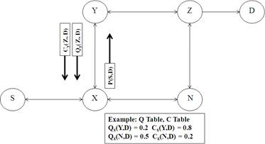
Figure 2. Q routing Including Confidence Measure.
3. Enhanced Confidence Based Q Routing
In Confidence based Q Routing Algorithm, the updating rule for a non-selected Q value is updating its C value with a decay constant value – λ. Also it is necessary that learning rate discussed before should not be constant and should change based on different network conditions [10,11].
If Q value changes (means the selected Q value is higher than the others) then it will select a new node having minimum Q value. As illustrated in figure 3(a), Node A has two neighbors, one neighbor who is selected for transmission as next hop to some destination, while other one is non-selected node. The node having Q value not selected for long duration, corresponding C value decays and thus corresponding Q value becomes unreliable [11].
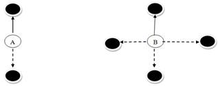
Figure 3. Node A and Node B with two and four node connections respectively.
As illustrated in figure 3(b), where B has four nodes, 3 nodes whose Q value not selected for long time, thus unselected nodes becomes more unreliable to transmit packets. Node A may not need to have a high learning rate as compared to node B since node A is updating its Q values more frequently compared to node B. In other words, node B has to have a higher learning rate according to the first rule of learning rate function because it has lower confidence since it has longer waiting time to update all its Q values.
A simple solution is by introducing the Variable of Decay Constant Approach. Thus for non-selected connections the decay constant will be λ{1-(n-1)} where n >=2, where n is the number of node connections. [11]
Thus update rule for selected connection will be
Cx(Y, D)new = Cx(Y, D)old + max (CY(Z, D), 1 - Cx(Y, D)old) * (CY(Z, D) - Cx(Y, D)old) (9)
The update rule for non-selected connection will be
Cx(Z, D)new = λ{1-(n-1)} Cx(Z, D)old (10)
where Z is non-selected neighboring node.
The reliability of the Q value is determined by the C value. A C value of one indicates that the Q value is completely reliable since it has just been updated. A value of zero for C value states that the Q value is completely unreliable since it has not been updated for quite some time [11].
The confidence value is never used for selecting routing policy in CQ routing; instead routing policy solely depends on Q value. Confidence value is only used to indicate reliability of Q value. If the C value equals to one, it has two possibilities: it has previously been updated or the packet will reach its destination in the next step. When the C value equals to one, we assume that this numeric Q value reflects 100% of the actual state of the network [11].
When the C value reduces, for instance to 0.95, we can assume that the Q value reflects approximately 95% of the actual state of the network. So, the Q value is about ± 5% disparate from the actual state. From the above assumptions, a C value of 0.95 for estimated Q value therefore reflects that the actual state is ±5% from the current Q value. It is better to test a value 5% lower instead of 5% higher. The additional 5% will make the Q value larger and less likely to get updated. It could be argued that when the C value equals to zero, then the Q value will be zero. This does not really reflect the actual situation. In fact, this is true but it is a positive errand number for the Q value. Such is the case because the decision maker will choose this errand number in a shorter time and the error will be corrected (at the same time updating this random Q value). Using this approach, the non-selected Q values are more competitive for selection and more exploration will occur [11].
These non-selected Q values will be updated as follows:
Qx(Z, D)new = Qx(Z, D)old – {(1- Qx(Z, D)new ) Qx(Z, D)old (11)
where Z is the non-selected node.
4. Analysis of Various Reinforcement Based Routing Methods
In order to see the effects of ECQ routing, two different experiements are performed. In first experiment ECQ routing is compared with shortest path routing (fixed network routing protocol), simple reinforcement and CQ routing. In second experiment, ECQ routing is compared with existing routing protocols such as DSDV, AODV and DSR. Simulation parameters used in first experiment and second experiment are mentioned in Table 1 and Table 2 respectively.
Table 1. Simulation Parameters Used for Experiment 1.
| Parameter | Value |
| Number of nodes | 50 Nodes |
| Simulation time | 200s |
| Topology Size | 1000×1000 |
| Initial Energy | 100 Joules |
| Packet Size | 2000 bytes |
| Interval | 0.6 to 1.0 increment by 0.1 |
| Routing protocols analysed | Shortest Path Routing, Reinforcement Routing, CQ Routing, ECQ Routing |
| Analysed Parameters | Packet Delivery Ratio, Delay, Control Overhead, Throughput etc |
Packet delivery ratio (PDR) is the ratio of the number of delivered data packet to the destination. The result of Packet delivery ratio is illustrated in Figure 4. Enhanced CQ Routing is compared with shortest path routing, reinforcement routing and with CQ routing. The intervals between the successive packets are changed to see the effects on mentioned parameters. The shortest path routing designed for wired network are not suitable for ad hoc networks because of special characteristics of ad hoc network such as Multihopping, mobility etc. CQ routing performance is better than reinforcement routing as it also includes confidence values for reliability of Q values. ECQ routing will provide the good results and PDR lies somewhere at 90% and remains throughout constant.
Table 2. Simulation Parameters Used for Experiment 2.
| Parameter | Value |
| Number of nodes | 10 Nodes to 100 Nodes |
| Simulation time | 200s |
| Topology Size | 1000×1000 |
| Initial Energy | 100 Joules |
| Mobility Model | Random Waypoint Mobility Model |
| Routing protocols analysed | DSDV, AODV, DSR and ECQ Routing |
| Analysed Parameters | Packet Delivery Ratio, Delay, Control Overhead, Throughput etc |
The result of Packet delivery ratio is illustrated in Figure 5. It is observed that when the network size increases beyond 60 nodes, AODV or DSR protocols starts dropping packets. But ECQ routing protocol maintains consistent ratio throughout the network irrespective of the network size. Thus almost 95% PDR is obtained.
Table 3 specifies the comparative analysis of packet delivery ratio for different routing protocols with ECQ routing in NS2.
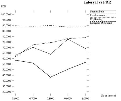
Figure 4. Interval vs. PDR.
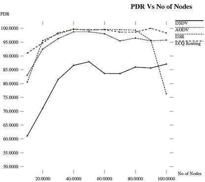
Figure 5. PDR vs. No of Nodes.
Table 3. Comparative analysis of PDR.
| No of Nodes | 10 | 20 | 30 | 40 | 50 | 60 | 70 | 80 | 90 | 100 |
| DSDV | 61.05 | 71.05 | 81.48 | 86.57 | 87.89 | 83.65 | 83.60 | 85.95 | 85.63 | 87.04 |
| AODV | 83.03 | 92.46 | 96.25 | 98.70 | 98.73 | 97.99 | 95.43 | 96.43 | 95.43 | 95.75 |
| DSR | 80.48 | 95.53 | 97.95 | 99.74 | 99.33 | 99.56 | 99.47 | 99.34 | 95.64 | 76.30 |
| ECQ | 91.02 | 94.73 | 98.38 | 99.54 | 99.47 | 99.47 | 98.62 | 98.61 | 100 | 98.30 |
End-to-end Delay is the time taken by a data packet to reach to the destination. The result of end to end delay for experiment 1 is illustrated in Figure 6. ECQ routing will provide minimum delay for the packets to reach to the destination.
The result of end to end delay for experiment 2 is illustrated in Figure 7. DSDV is the proactive routing protocol which always provides minimum delay, AODV and DSR protocols are on demand routing routing protocols hence they took more delay for route discovery process. ECQ routing provides alternate path whenever required and thus takes care that packet reaches to the destination in minimum amount of time.
Table 4 specifies the comparative analysis of delay in ms for different routing protocols with ECQ routing in NS2.
Control overhead is defined as the total number of control messages and control packets generated by each node throughout the network. As in ECQ routing, confidence values are used to indicate reliability of Q values and also due to update All Q value approach, less time is needed to represent real state of the network and thus less control packets are generated as compared with traditional approach. The result of control overhead over varying number of intervals is illustrated in Figure 8.
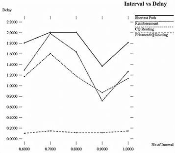
Figure 6. No of Nodes Vs Delay.
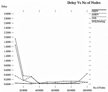
Figure 7. Delay Vs No of Nodes.
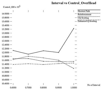
Figure 8. Interval vs. Control Overhead.
Table 4. Comparative analysis of Delay vs No of Nodes.
| No of Nodes | 10 | 20 | 30 | 40 | 50 | 60 | 70 | 80 | 90 | 100 |
| DSDV | 0.047 | 0.029 | 0.013 | 0.051 | 0.031 | 0.025 | 0.024 | 0.022 | 0.028 | 0.028 |
| AODV | 1.666 | 0.169 | 0.057 | 0.031 | 0.094 | 0.090 | 0.123 | 0.125 | 0.122 | 0.073 |
| DSR | 1.931 | 0.357 | 0.325 | 0.017 | 0.039 | 0.026 | 0.033 | 0.031 | 0.132 | 0.452 |
| ECQ | 0.359 | 0.158 | 0.317 | 0.030 | 0.019 | 0.058 | 0.037 | 0.069 | 0.041 | 0.088 |
The result of control overhead over varying number of nodes is illustrated in Figure 9. It is found that DSDV generates less number of control packets due to their proactive nature. AODV and DSR protocols due to their on demand nature generate large number of control packets. Every time when path between source node and destination node breaks down, router discovery process is carried out; this request propagates throughout the network and thus reaches to the destination. In ECQ routing, control packet is generated at every time when data packet is transmitted from one node to the next node. But the size of the control packet is less; hence control overhead is less as compared with existing routing protocols.
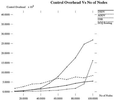
Figure 9. Control Overhead vs. No of Nodes.
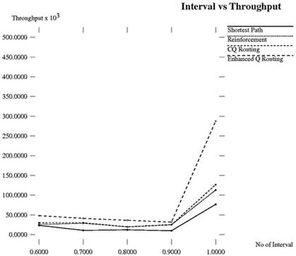
Figure 10. Interval vs. Throughput.
Table 5 specifies the comparative analysis of control overhead for different routing protocols with ECQ routing in NS2.
Throughput is the amount of data received by the destination. The throughput is usually measured in bits per second or data packets per time slot. The result of throughput for experiment 1 is illustrated in Figure 10.
The result of throughput for experiment 1 is illustrated in Figure 10. The result of throughput for experiment 2 is illustrated in Figure 11. Table 6 specifies the comparative analysis of throughput (106) for different routing protocols with ECQ routing in NS2.
Table 5. Comparative analysis of Control Overhead.
| No of Nodes | 10 | 20 | 30 | 40 | 50 | 60 | 70 | 80 | 90 | 100 |
| DSDV | 182 | 484 | 1004 | 1383 | 2051 | 2615 | 3314 | 4328 | 5053 | 5476 |
| AODV | 307 | 570 | 1025 | 1894 | 4432 | 7887 | 12804 | 17553 | 24663 | 26850 |
| DSR | 114 | 103 | 195 | 381 | 565 | 727 | 1297 | 1721 | 4066 | 16158 |
| ECQ | 1727 | 2637 | 3979 | 4242 | 5487 | 6970 | 6316 | 7619 | 7230 | 8394 |
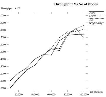
Figure 11. Throughput vs. No of Nodes.
Table 6. Comparative analysis of Throughput vs No of Nodes.
| No of Nodes | 10 | 20 | 30 | 40 | 50 | 60 | 70 | 80 | 90 | 100 |
| DSDV | 104480 | 209120 | 278560 | 400640 | 461920 | 455360 | 653280 | 727520 | 739280 | 742285 |
| AODV | 2400 | 133600 | 247040 | 317440 | 450880 | 540000 | 515520 | 731680 | 816800 | 865120 |
| DSR | 6560 | 140480 | 252960 | 315680 | 455680 | 549280 | 546080 | 747840 | 817920 | 689280 |
| ECQ | 8800 | 140960 | 252800 | 317120 | 454240 | 548000 | 695360 | 774080 | 780800 | 811252 |
5. Conclusion
This paper explains the optimization of Confidence based Q routing – Enhanced Q routing and compares the performance with existing routing protocols. This research study compares DSDV, AODV and DSR protocols with ECQ routing protocols for an ad hoc network. PDR and delay are very important parameters when deciding how a reliable a protocols works. In our simulation environment PDR and delay in ECQ routing outperforms AODV and DSR routing protocols with almost 95-100% without packet loss with lower delay. In this paper, we proposed enhancement in CQ routing along with the forward exploration and confidence measure called as enhanced Q routing.
References
- Asma Toteja, Raynees Gujral, Sunil Thalia, "Comparative performance Analysis of DSDV, AODV and DSR Routing Protocols in MANETs, using NS2", 2010 International Conference on Advances in computing Engineering, IEEE Computer Society.
- Khan, K.; Zaman, R.U.; Reddy, K.A.; Reddy, K.A.; Harsha, T.S., "An Efficient DSDV Routing Protocol for Wireless Mobile Ad Hoc Networks and its Performance Comparison," Second UKSIM European Symposium on Computer Modeling and Simulation, 2008. EMS '08. , pp.506,511, 8-10 Sept. 2008
- Bai, R.; Singhal, M., "DOA: DSR over AODV Routing for Mobile Ad Hoc Networks," Mobile Computing, IEEE Transactions on , vol.5, no.10, pp.1403,1416, Oct. 2006
- D B Johnson, D A Maltz, Y. Hu and J G Jetcheva. The Dynamic Source Routing Protocol for Mobile Ad Hoc Networks (DSR) http://www.ietf.org/internet-drafts/draft-ietf-manet-dsr-07.txt, Feb 2002, IETF Internet Draft.
- Richard S. Sutton and Andrew G. Barto "Reinforcement Learning: An Introduction" A Bradford Book, The MIT Press Cambridge, Massachusetts London, England
- Ramzi A. Haraty and Badieh Traboulsi "MANET with the Q-Routing Protocol" ICN 2012: The Eleventh International Conference on Networks
- S Kumar, Confidence based Dual Reinforcement Q Routing : An on line Adaptive Network Routing Algorithm. Technical Report, University of Texas, Austin 1998.
- Kumar, S., 1998, "Confidence based Dual Reinforcement Q-Routing: An On-line Adaptive Network Routing Algorithm," Master’s thesis, Department of Computer Sciences, The University of Texas at Austin, Austin, TX-78712, USA Tech. Report AI98-267.
- Kumar, S., Miikkulainen, R., 1997, "Dual Reinforcement Q-Routing: An On-line Adaptive Routing Algorithm," Proc. Proceedings of the Artificial Neural Networks in Engineering Conference.
- Shalabh Bhatnagar, K. Mohan Babu "New Algorithms of the Q-learning type" Science Direct Automatica 44 (2008) 1111- 1119. Website: www.sciencedirect.com.
- Soon Teck Yap and Mohamed Othman, "An Adaptive Routing Algorithm: Enhanced Confidence Based Q Routing Algorithms in Network Traffic.Malaysian Journal of Computer, Vol. 17 No. 2, December 2004, pp. 21-29


