
Physics Journal, Vol. 1, No. 2, September 2015 Publish Date: Jul. 25, 2015 Pages: 35-44
Single Electron Tunneling Between Conducting Half-Space and Three-Dimensional Potential Well Through an Inhomogeneous Barrier, Described by Dirac Delta Function
N. V. Khotkevych*, Yu. A. Kolesnichenko
B.I. Verkin Institute for Low Temperature Physics and Engineering, National Academy of Sciences of Ukraine, Kharkiv, Ukraine
Abstract
This paper is dedicated to further development of the theory of the current states in small size tunnel contacts. We have consistently investigated the problem of electron tunneling through an inhomogeneous barrier, which is described by Dirac delta function, between a conducting half-space, and a three-dimensional quantum well. The electron tunneling from the states with the continuous energy spectrum into the quantized states of the three-dimensional potential well is considered as well as the tunneling in the opposite direction. In order to solve the above problem we develop an original method based on the asymptotical expansion of the electron wave function in small parameter, could be defined by means of characteristic radius of the transmission region and an amplitude of the tunnel barrier. The key advantage of our method is in its ability to determine the system properties in the asymptotically explicit way. Following our approach we describe the tunnel current in such systems as a function of the system parameters. The results can be used for interpretation of experiments in scanning tunneling microscopy.
Keywords
Electron Tunneling, Tunnel Current, Conductance, STM, Inhomogeneous Barrier
Received: June 19, 2015
Accepted: July 10, 2015
Published online: July 24, 2015
@ 2015 The Authors. Published by American Institute of Science. This Open Access article is under the CC BY-NC license. http://creativecommons.org/licenses/by-nc/4.0/
1. Introduction
The problem of quantum-mechanical tunneling through a spatially inhomogeneous barrier is of great interest in regard of the scanning tunneling microscopy (STM) [1-4]. From the mathematical point of view the problem lies in the solution of three-dimensional Schrödinger equation with the boundary conditions given at the flat interface ![]() (surface of a sample) and at the sharp interface
(surface of a sample) and at the sharp interface ![]() (surface of the STM tip) (see Fig. 1a). Generally, the tunneling occurs through a small region between the tip apex and a part of the surface underneath. To the best of our knowledge, there are no exact or asymptotically exact analytical solutions of this problem for any realistic three-dimensional model of the STM tip (Fig. 1a) published to date. The demand for a description of the conductance measured by the STM is partly addressed by exploiting numerical calculations [5] or by use of certain model wave functions which in their absolute majority do not satisfy all the boundary conditions simultaneously [6,7]. That is why a search for the exact (or asymptotically exact) solutions of the described problem for various models of the spatially inhomogeneous barrier is important.
(surface of the STM tip) (see Fig. 1a). Generally, the tunneling occurs through a small region between the tip apex and a part of the surface underneath. To the best of our knowledge, there are no exact or asymptotically exact analytical solutions of this problem for any realistic three-dimensional model of the STM tip (Fig. 1a) published to date. The demand for a description of the conductance measured by the STM is partly addressed by exploiting numerical calculations [5] or by use of certain model wave functions which in their absolute majority do not satisfy all the boundary conditions simultaneously [6,7]. That is why a search for the exact (or asymptotically exact) solutions of the described problem for various models of the spatially inhomogeneous barrier is important.
One of the possible candidates for description of STM experiments is the model of inhomogeneous ![]() - barrier [8-10]. In this model the barrier potential is given by the function
- barrier [8-10]. In this model the barrier potential is given by the function
where ![]() is an arbitrary function of two-dimensional vector r=(x,y) which satisfies the conditions
is an arbitrary function of two-dimensional vector r=(x,y) which satisfies the conditions
![]() (2)
(2)
The length ![]() plays a role of the contact radius.
plays a role of the contact radius.
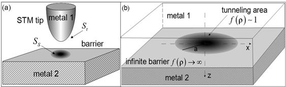
Fig. 1. Schematic of a STM device (a), and the model of inhomogeneous dielectric ![]() - barrier between two metals (b).
- barrier between two metals (b).
In the paper [5] the Schrödinger equation with the potential (1) was solved asymptotically exactly in ![]() for the tunneling between two equivalent half-spaces, and the tunnel current of the system was found. The case of the arbitrary barrier amplitude
for the tunneling between two equivalent half-spaces, and the tunnel current of the system was found. The case of the arbitrary barrier amplitude ![]() was analyzed in the works [6,7]. Authors of the publication [11] proposed to use the model of inhomogeneous
was analyzed in the works [6,7]. Authors of the publication [11] proposed to use the model of inhomogeneous ![]() - barrier (1) of low transparency to describe the influence of a single subsurface defect on the STM-conductance (for review see Ref. [12]). Later on [13,14]this model was applied for the interpretation of experimental results on scanning tunneling spectroscopy of thin films [10] and anisotropic surface states [11]. However, the consistent mathematical solution of the problem of single-particle tunneling between half-space and three-dimensional potential well through the inhomogeneous
- barrier (1) of low transparency to describe the influence of a single subsurface defect on the STM-conductance (for review see Ref. [12]). Later on [13,14]this model was applied for the interpretation of experimental results on scanning tunneling spectroscopy of thin films [10] and anisotropic surface states [11]. However, the consistent mathematical solution of the problem of single-particle tunneling between half-space and three-dimensional potential well through the inhomogeneous ![]() - barrier, was not presented in Refs. [10,11].
- barrier, was not presented in Refs. [10,11].
In this paper, we describe the mathematical scheme of finding the asymptotically exact solution of the mentioned problem in the limit ![]() ,
, ![]() that corresponds to typical parameters of the STM. The mathematically rigorous asymptotic solutions for the wave functions transmitted through the barrier are found for the both directions of electron tunneling, and the tunnel current in the system is calculated. We demonstrate that our solutions satisfy all the necessary boundary conditions and provide the conservation of total current flow through any surface overlapping the contact region. From the point of view of the theoretical physics, we show how a three-dimensional electron wave from the semi-bounded conductor is transformed after tunneling into a surface one and vice versa.
that corresponds to typical parameters of the STM. The mathematically rigorous asymptotic solutions for the wave functions transmitted through the barrier are found for the both directions of electron tunneling, and the tunnel current in the system is calculated. We demonstrate that our solutions satisfy all the necessary boundary conditions and provide the conservation of total current flow through any surface overlapping the contact region. From the point of view of the theoretical physics, we show how a three-dimensional electron wave from the semi-bounded conductor is transformed after tunneling into a surface one and vice versa.
2. The Model and Mathematical Formulation of the Problem
The model used for solving the problem is presented at Fig.1b. Electrons can tunnel through a finite area (centered at the point ![]() ) in an infinitely thin insulating layer
) in an infinitely thin insulating layer ![]() between two conducting half-spaces. We describe the barrier potential as
between two conducting half-spaces. We describe the barrier potential as ![]() (1), where
(1), where ![]() is an analytical steadily increasing function. A simple example of such a barrier (1) is the following exponential function
is an analytical steadily increasing function. A simple example of such a barrier (1) is the following exponential function
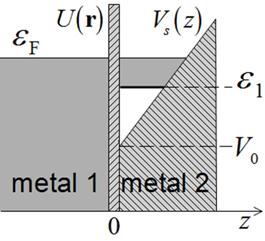
Fig. 2. Energy zones in half-space (metal 1) and potential well (metal 2) at zero voltage. The occupied states are shaded.
The potential ![]() exists in the half-space
exists in the half-space ![]() . Together with the barrier (1) it forms the three-dimensional potential well
. Together with the barrier (1) it forms the three-dimensional potential well ![]() (see. Fig. 2). For the sake of simplicity and for carrying out further calculations explicitly we use the model of linear potential
(see. Fig. 2). For the sake of simplicity and for carrying out further calculations explicitly we use the model of linear potential
The Schrödinger equation of our system is written as
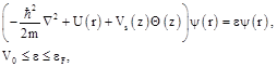
where ![]() ,
, ![]() and
and ![]() are the electron energy, the absolute value of the wave vector and the electron mass, respectively,
are the electron energy, the absolute value of the wave vector and the electron mass, respectively, ![]() is the maximum value of the electron energy in metal at zero temperature (Fermi energy). At the interface
is the maximum value of the electron energy in metal at zero temperature (Fermi energy). At the interface ![]() the wave function
the wave function ![]() satisfies the continuity condition
satisfies the continuity condition
and also the condition of finite jump in the normal derivative, which is caused by the shape of the potential barrier (1)
We will follow the way of solution of Eq. (5) with the boundary conditions (6), (7) which was proposed in Ref. [5]. Desired wave functions ![]() are expanded into series in small parameter
are expanded into series in small parameter ![]()
where the functions ![]() are standing waves which correspond to a non-transparent interface and satisfy zero boundary condition
are standing waves which correspond to a non-transparent interface and satisfy zero boundary condition
Here and below the upper index ![]() signifies half-space
signifies half-space ![]() or
or ![]() .
.
Substituting the expansion (8) into the boundary conditions (6), (7) and equating the terms of zero order in ![]() (
(![]() does not depend on
does not depend on ![]() ) we get the reduced boundary conditions
) we get the reduced boundary conditions
![]() (10)
(10)
The relation (11) converts the problem of finding the wave function of transmitted electrons ![]() in the linear in
in the linear in ![]() approximation into a more simple task of finding the wave functions
approximation into a more simple task of finding the wave functions ![]() in half-spaces and subsequent solution of the Schrödinger equation (5) for
in half-spaces and subsequent solution of the Schrödinger equation (5) for ![]() with value
with value ![]() at the interface given by Eq. (11).
at the interface given by Eq. (11).
For calculation of the tunnel current, it is enough to know the wave function ![]() of transmitted particles.
of transmitted particles.
The model, in which tunneling is possible only inside limited layer near ![]() - barrier, substantially differs from the model of two equivalent half-spaces, considered in the paper [5]. In the mentioned work at
- barrier, substantially differs from the model of two equivalent half-spaces, considered in the paper [5]. In the mentioned work at ![]() , the formula for the tunneling current becomes the classical expression for the current flowing through a homogeneous barrier of low transparency. In the considered system the electron motion in the
, the formula for the tunneling current becomes the classical expression for the current flowing through a homogeneous barrier of low transparency. In the considered system the electron motion in the ![]() -axis direction is confined (Fig.2), and in the case of homogenous barrier (
-axis direction is confined (Fig.2), and in the case of homogenous barrier (![]() ) the tunneling current is absent.
) the tunneling current is absent.
We show below that in the case of inhomogeneous barrier the total flux through the area of non-zero transparency (contact) is non-zero, and thus, the system has non-zero tunnel current. The perturbation theory is applicable to this problem only for the contacts of sufficiently small radius ![]() when the dimensionless small parameter of the theory satisfies the condition
when the dimensionless small parameter of the theory satisfies the condition
where ![]() is the electron Fermi wave vector,
is the electron Fermi wave vector, ![]() is the characteristic depth of localization of the wave function at
is the characteristic depth of localization of the wave function at ![]() due to the potential (4).
due to the potential (4).
3. Tunnelling from the Half-Space into the Potential Well
Let us begin our consideration with the case when an electron tunnels from the half-space ![]() into the bounded states in the half-space
into the bounded states in the half-space![]() . The wave function in zero approximation in
. The wave function in zero approximation in ![]() has the form
has the form
 (14)
(14)
where ![]() and
and ![]() are tangential and normal to interface
are tangential and normal to interface ![]() components of the wave vector. In the first approximation on
components of the wave vector. In the first approximation on ![]() the wave functions at
the wave functions at ![]() and
and ![]() are written as
are written as
![]() (15)
(15)
Substituting Eqs. (13) into the reduced boundary condition (7) we get the condition [5]:
which is valid at ![]() and
and ![]() .
.
The boundary conditions for ![]() at
at ![]() are defined by
are defined by
1) the wave function damping in the classically forbidden region,
![]() and (18)
and (18)
2) the existence of two-dimensional waves diverging from the center ![]() ,
,
We expand the function ![]() in the Fourier integral in
in the Fourier integral in ![]()
Substituting the expansion (20) into Eq. (5) and taking into account the zero condition (18) at ![]() , we find
, we find
where ![]() is Airy function,
is Airy function, ![]() ,
,
the length ![]() plays the role of a characteristic depth of localization of the bounded state near the interface. Fourier components (21) tend to zero at
plays the role of a characteristic depth of localization of the bounded state near the interface. Fourier components (21) tend to zero at ![]() or
or ![]() . The inverse transform of expression (21) together with Eq.(17) at
. The inverse transform of expression (21) together with Eq.(17) at ![]() gives the relation:
gives the relation:
which allows us to determine the function ![]() under the assumption that
under the assumption that ![]() .
.
The Airy function ![]() has an infinite number of zeros
has an infinite number of zeros ![]() , all of which are negative. We assume that for a given value
, all of which are negative. We assume that for a given value ![]() only one (minimal) value
only one (minimal) value ![]() exists, for which
exists, for which ![]() , where
, where ![]() is the first zero.
is the first zero.
From Eq. (22) we find that
![]() (24)
(24)
where
is the first energy level for electron in the triangular potential well, which is formed by the potential (4) and infinite wall at ![]() .
.
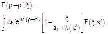
We represent the function ![]() by Fourier transform of the function
by Fourier transform of the function ![]() in
in ![]() , getting the discontinuity of the second kind at the point
, getting the discontinuity of the second kind at the point ![]()
where
In Eq. (27) and below ![]() are the Bessel functions. It is easy to see that the function
are the Bessel functions. It is easy to see that the function ![]() (26) satisfies the boundary condition (17). The Eq.(26) becomes the solution for a homogeneous barrier, for which the current is zero. It is clear that for any
(26) satisfies the boundary condition (17). The Eq.(26) becomes the solution for a homogeneous barrier, for which the current is zero. It is clear that for any ![]() and
and ![]() at
at ![]() the function
the function ![]() , and there is a certain interval of small
, and there is a certain interval of small ![]() , for which the amplitude of the wave function
, for which the amplitude of the wave function ![]() (26) for transmitted electrons remains small in comparison with the amplitude of the incident wave. The latter makes the perturbation theory applicable.
(26) for transmitted electrons remains small in comparison with the amplitude of the incident wave. The latter makes the perturbation theory applicable.
At ![]() the integral (27) diverges because the integrand has a simple pole
the integral (27) diverges because the integrand has a simple pole ![]() inside the integration interval. Thus, Eq. (27) has a sense as a Cauchy Principal Value only.
inside the integration interval. Thus, Eq. (27) has a sense as a Cauchy Principal Value only.
The analytical function ![]() at
at ![]() can be written in the form
can be written in the form
in which ![]() . Substituting the Eq. (28) in the integrand of the Eq. (27) we rewrite it in the form
. Substituting the Eq. (28) in the integrand of the Eq. (27) we rewrite it in the form
were
According to Eq. (29) the wave function (26) can be divided into two parts
![]() (31)
(31)
where
with
and
with
Thus, the function ![]() (32) satisfies the boundary conditions (17), (18) and according to Eq. (A1.7)
(32) satisfies the boundary conditions (17), (18) and according to Eq. (A1.7)
![]() (36)
(36)
while ![]() (34) satisfies the conditions (18), (19) and it is vanishes at
(34) satisfies the conditions (18), (19) and it is vanishes at ![]() .
.
The total tunnel current ![]() can be calculated by integrating the charge flow over the wave vectors
can be calculated by integrating the charge flow over the wave vectors ![]() of the electrons incident on the boundary and by integration over any surface
of the electrons incident on the boundary and by integration over any surface ![]() overlapping the contact. If we choose the plane
overlapping the contact. If we choose the plane ![]() as the surface of integration, the current
as the surface of integration, the current ![]() is written as
is written as
 (37)
(37)
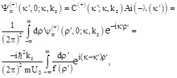
Let us write the wave function (26) under the assumptions ![]() . Using the results for
. Using the results for ![]() (A1.13) and
(A1.13) and ![]() (A2.4) the Eq. (26) at
(A2.4) the Eq. (26) at ![]() takes the form
takes the form
were
![]() (39)
(39)
and
![]() (40)
(40)
We evaluate the electrical current at zero temperature and in the Ohm’s law approximation, which is true if ![]() (
(![]() is the voltage applied to the tunnel contact). Respectively, in such a case it is enough to know the electron wave function
is the voltage applied to the tunnel contact). Respectively, in such a case it is enough to know the electron wave function ![]() of electrons transmitted through the barrier at
of electrons transmitted through the barrier at ![]() . A positive sign of the energy bias
. A positive sign of the energy bias ![]() corresponds to the possibility of electron tunneling from the occupied states in the half-space
corresponds to the possibility of electron tunneling from the occupied states in the half-space ![]() into bounded states in the half-space
into bounded states in the half-space ![]() (Fig. 2). At
(Fig. 2). At ![]() tunneling occurs in the opposite direction.
tunneling occurs in the opposite direction.
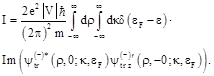
The total tunnel current ![]() can be calculated by integrating the charge flow over the wave vectors
can be calculated by integrating the charge flow over the wave vectors ![]() of the electrons incident on the boundary and by integration over any surface
of the electrons incident on the boundary and by integration over any surface ![]() overlapping the contact. If we choose the plane
overlapping the contact. If we choose the plane ![]() as the surface of integration, the current
as the surface of integration, the current ![]() is written as
is written as
 (41)
(41)
In Eq. (30) ![]() and
and ![]() are the angles of the spherical coordinate system in the
are the angles of the spherical coordinate system in the ![]() - space. Evaluating the integrals, we obtain the following expression for the current
- space. Evaluating the integrals, we obtain the following expression for the current
where ![]() is the spherical Bessel function. The Eq. (42) makes it possible to find the linear conductance of the system
is the spherical Bessel function. The Eq. (42) makes it possible to find the linear conductance of the system ![]() .
.
The requirement of conservation of the total current I means that the above result has to be insensitive to the choice of the surface over which the integration in (42) is carried out. This provides a way of verifying the obtained expression. Let us calculate the current, for example, by integrating over the surface of an infinite cylinder of radius ![]() with the axis along
with the axis along ![]() :
:
where ![]() is the azimuth in the cylindrical coordinate system in real space. The integration can be performed easily by considering an infinite cylinder of large diameter
is the azimuth in the cylindrical coordinate system in real space. The integration can be performed easily by considering an infinite cylinder of large diameter ![]() and by using the asymptotic behavior of the Hankel function
and by using the asymptotic behavior of the Hankel function
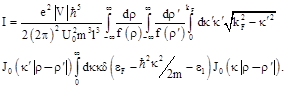
Substituting the asymptotic formula (44) in Eq. (43), we obtain:
The integrals over the variables ![]() ,
, ![]() ,
, ![]() and
and ![]() can be calculated exactly and we come once again to the formula (42) for the current.
can be calculated exactly and we come once again to the formula (42) for the current.
4. Tunnelling from the Potential Well into the Half-Space
Let us now consider the opposite direction of the current, which corresponds to the tunneling of electrons from the bounded state in the potential well into the half-space ![]() . In this case, the wave functions of the zero-order approximation in
. In this case, the wave functions of the zero-order approximation in ![]() (12) can be found by using solutions of the Schrödinger equation for a triangular potential well
(12) can be found by using solutions of the Schrödinger equation for a triangular potential well
and the reduced boundary condition (11), which in this case takes the form
Wave function (46) is normalized
![]() (48)
(48)
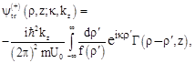
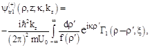
We represent the wave function ![]() of the electrons transmitted into the half-space
of the electrons transmitted into the half-space ![]() electrons as Fourier integral
electrons as Fourier integral
![]() (49)
(49)
where, as follows from the Schrödinger equation, the coefficients ![]() can be written in the form:
can be written in the form:
![]() at
at ![]() . The sign in the exponent in (50) is dictated by the requirement of the existence of the diverging three-dimensional waves at
. The sign in the exponent in (50) is dictated by the requirement of the existence of the diverging three-dimensional waves at ![]() :
:
![]() (51)
(51)
Using the boundary condition (47), we find the function ![]() :
:
 (52)
(52)
As a result, one can derive the following expression for the wave function of transmitted electrons:
It is easy to check that at ![]() the function (53) satisfies the boundary condition (47). The integral over
the function (53) satisfies the boundary condition (47). The integral over ![]() in equation (53) can be calculated at
in equation (53) can be calculated at ![]()
where ![]() is a spherical Hankel function, and
is a spherical Hankel function, and ![]() . Substituting the result of the integration (54) in Eq. (53) we finally find the expression, which is completely analogous to the Rayleigh – Sommerfeld diffraction formula [15, 16].
. Substituting the result of the integration (54) in Eq. (53) we finally find the expression, which is completely analogous to the Rayleigh – Sommerfeld diffraction formula [15, 16].
Similarly to the previous case, the tunneling current can be calculated by integrating the charge flow over coordinate ![]() in the plane
in the plane![]() and by integrating over the two-dimensional wave vector
and by integrating over the two-dimensional wave vector ![]() :
:
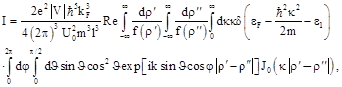
Substituting the wave function ![]() (53) and its derivative at
(53) and its derivative at ![]() in the expression for the current (55) one can obtain
in the expression for the current (55) one can obtain
After exact integration over variables ![]() (by means of
(by means of ![]() - function and
- function and ![]() ) we get the expression (42).
) we get the expression (42).
Solution (53) satisfies the condition of conservation of the total current through any surface covering the contact. For example, the current can be calculated by integrating over the hemisphere of radius ![]()
where ![]() ,
, ![]() are the angles in the spherical coordinate system in real space. Using the asymptotic form of the wave functions (53) at large
are the angles in the spherical coordinate system in real space. Using the asymptotic form of the wave functions (53) at large ![]() (
(![]() )
)
 (58)
(58)
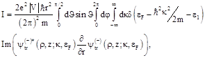
we transform the Eq. (57)
 (59)
(59)
and after integrations we finally get the result (42).
5. Limit of Ultra Small Contact
Let us consider the case of a very small contact ![]() . Substituting the model function
. Substituting the model function ![]() (3) in the Eq. (38) in the limit
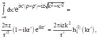
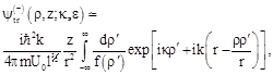
(3) in the Eq. (38) in the limit ![]() for
for ![]() we find the asymptotic formula for the wave function of electrons transmitted into the potential well
we find the asymptotic formula for the wave function of electrons transmitted into the potential well
Expression (53) for the wave function of electrons tunneling from the potential well to the half-space at ![]() and
and ![]() takes the form:
takes the form:
where ![]() .
.
Thus we have found the wave functions outside the contact area ![]() at the interface
at the interface ![]() between conductors, which satisfy the zero boundary condition
between conductors, which satisfy the zero boundary condition ![]() at
at ![]() . These functions are concentric surface waves (60) or spherical bulk waves (61), depending on the direction of tunneling. Despite significantly different character of the current spreading, as we have seen, the total current through the contact does not depend on the direction of tunneling.
. These functions are concentric surface waves (60) or spherical bulk waves (61), depending on the direction of tunneling. Despite significantly different character of the current spreading, as we have seen, the total current through the contact does not depend on the direction of tunneling.
In the given case of a small contact ![]() formula for the current (42) is reduced to:
formula for the current (42) is reduced to:
6. Conclusions
Thus, for the model of inhomogeneous ![]() - barrier of arbitrary shape and large amplitude we found asymptotically exact expressions for the wave functions
- barrier of arbitrary shape and large amplitude we found asymptotically exact expressions for the wave functions ![]() transmitted through the barrier in the case of tunneling between the half-space and the three-dimensional well. The obtained result (42) gives the dependence of the tunnel current on the form and amplitude of the potential barrier and on the parameters of the electron energy spectrum (the effective mass and the Fermi wave vector) as well as the characteristic depth of localization of the surface states. The listed values can be easily estimated in STM experiments. In addition our results can be employed in the theory of the light diffraction by a plane aperture. Despite the fact that the latter problem has been intensely investigated since the pioneering works performed in the 18th century, it still attracts attention of mathematicians and physicists (see, for example, Refs. [17-20]).
transmitted through the barrier in the case of tunneling between the half-space and the three-dimensional well. The obtained result (42) gives the dependence of the tunnel current on the form and amplitude of the potential barrier and on the parameters of the electron energy spectrum (the effective mass and the Fermi wave vector) as well as the characteristic depth of localization of the surface states. The listed values can be easily estimated in STM experiments. In addition our results can be employed in the theory of the light diffraction by a plane aperture. Despite the fact that the latter problem has been intensely investigated since the pioneering works performed in the 18th century, it still attracts attention of mathematicians and physicists (see, for example, Refs. [17-20]).
Appendix I
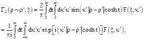
Let consider the integrand ![]() (33) of Eq. (32). After the integration over directions of vector
(33) of Eq. (32). After the integration over directions of vector ![]() it takes the form
it takes the form
were ![]() , which is given by Eq. (30), is the bounded analytical function of its arguments which has no singularities on intervals
, which is given by Eq. (30), is the bounded analytical function of its arguments which has no singularities on intervals ![]() ,
, ![]() , and
, and
At ![]() ,
, ![]() and
and
![]() (A1.3)
(A1.3)
Next, we use the representation of the Bessel function ![]() [21]
[21]
and rewrite the ![]() (A1.1) in the form of a double integral
(A1.1) in the form of a double integral
If ![]() , in accordance with Eq. (A1.2)
, in accordance with Eq. (A1.2) ![]() is an absolutely integrable function
is an absolutely integrable function
![]() (A1.6)
(A1.6)
and, as it follows from the Riemann–Lebesgue lemma,
The property (A1.7) provides a convergence of the double integral (32).
Under conditions ![]() and
and ![]() , the integral over
, the integral over ![]() can be calculated by using the theory of residues. According to Eqs. (28) and (30) the function
can be calculated by using the theory of residues. According to Eqs. (28) and (30) the function ![]() has infinite number of poles on the imaginary axis at
has infinite number of poles on the imaginary axis at
were
![]() (A1.9)
(A1.9)
After integration over a contour, which is shown in Fig.3, we find
Taking into account relations
![]() (A1.11)
(A1.11)
and
![]() (A1.12)
(A1.12)
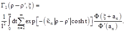
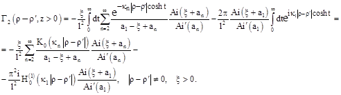
the Eq. (A1.10) can be rewritten in the form
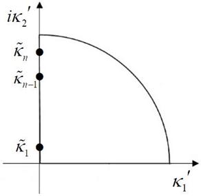
Fig. 3. The contour in ![]() plane for calculation of the improper integral (A1.5).
plane for calculation of the improper integral (A1.5).
The modified Bessel function of the second kind ![]() at large and small positive arguments has asymptotic behavior
at large and small positive arguments has asymptotic behavior
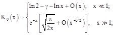
where ![]() is Euler constant. From Eq. (A1.14) it is follows that at
is Euler constant. From Eq. (A1.14) it is follows that at ![]() the function
the function ![]() monotonically (exponentially) vanishes, and at
monotonically (exponentially) vanishes, and at ![]() it has a logarithmic singularity.
it has a logarithmic singularity.
Appendix II
In this appendix, we analyze the integrand ![]() (35) of Eq. (34) under the assumption
(35) of Eq. (34) under the assumption ![]()
![]() (A2.1)
(A2.1)
Next, we use the representation of the Bessel function ![]() (A1.4) and rewrite
(A1.4) and rewrite ![]() in the form of a double integral
in the form of a double integral
![]() (A2.2)
(A2.2)
Further calculations are similar to finding the Green's function of a free particle (see, for example, Ref. [22,23]) or integrals which appear in scattering problems [5]. The integral (A2.2) is divergent and therefore ambiguous. From the boundary condition (19) the requirement for the solution (26) to represent the outgoing scattered wave at ![]() appears. Following the procedure described in Refs. [19,20] let us consider the loop integral
appears. Following the procedure described in Refs. [19,20] let us consider the loop integral
![]() (A2.3)
(A2.3)
over the contour presented in Fig.3, in which ![]() . This integral over
. This integral over ![]() is calculated by using the theory of residues. It is easy to check that the integrand satisfies Jordan's lemma, and the integral over the semicircle
is calculated by using the theory of residues. It is easy to check that the integrand satisfies Jordan's lemma, and the integral over the semicircle ![]() of radius
of radius ![]() tends to zero. The pole
tends to zero. The pole ![]() and the poles
and the poles ![]() (A1.8) occur inside the contour in Fig. 3. Taking into account that from Eq. (28) it follows
(A1.8) occur inside the contour in Fig. 3. Taking into account that from Eq. (28) it follows ![]() , we get:
, we get:
where ![]() is the Hankel function. At
is the Hankel function. At ![]() , Eq. goes to infinity
, Eq. goes to infinity
![]() (A2.5)
(A2.5)
Thus, the integrand ![]() in Eq. (26) has a single logarithmic singularity at the point
in Eq. (26) has a single logarithmic singularity at the point ![]() and the integral (26) converges.
and the integral (26) converges.
Acknowledgments
We would like to acknowledge useful discussions with A.N. Omelyanchouk and S.V. Kuplevakhsky.
References
- G. Binnig, H. Rohrer IBM J. of Res. and Dev. 30, 4 (1986).
- M. Bouhassoune,B. Zimmermann, P. Mavropoulos, D. Wortmann, P.H. Dederichs, S. Blügel, S. Lounis, arXiv:1411.7861v1 (2014).
- S. Müllegger, S. Tebi, A.K. Das, W. Schöfberger, F. Faschinger, R. Koch, PRL 113, 133001 (2014).
- J. Stirling, Beilstein J. Nanotechnol. 5, 337–345, (2014).
- W. A. Hofer, A. S. Foster, A. L. Shluger, Rev. Mod.Phys. 75, 1287 (2003).
- J. Tersoff, D. Hamann, Phys. Rev. Lett. 50 1998 (1983); Phys. Rev. B 31, 805 (1985).
- C.J. Chen, Phys. Rev. B, 65, 148 (1985); J. Vac. Sei. Technol.A 9 (1), 44 (1991).
- I. O. Kulik, Yu .N. Mitsai, A. N. Omel'yanchuk, Sov. Phys.-JETP 39, 514 (1974).
- V. Bezak.J. of Math. Phys. 48, 112108 (2007).
- V. Bezak,Appl. Surf. Sci. 254, 3630 (2008).
- Ye.S. Avotina, Yu.A. Kolesnichenko, A.N. Omelyanchouk, A.F. Otte, and J. M. van Ruitenbeek, Phys. Rev. B 71, 115430 (2005).
- Ye.S. Avotina, Yu.A. Kolesnichenko, and J.M. van Ruitenbeek, Low Temp. Phys. 37, 53 (2011).
- N.V. Khotkevych, Yu.A. Kolesnichenko, and J.M. van Ruitenbeek, Low Temp. Phys. 38, 503 (2012).
- N.V. Khotkevych, Yu.A. Kolesnichenko, and J.M. van Ruitenbeek, Low Temp. Phys. 39, 299 (2013).
- Lord Rayleigh, Philos. Mag. 43, 259 (1897).
- A. Sommerfeld Lectures on Theoretical Physics, vol 4: Optics (New York: Academic, 1954).
- A. S. Marathay and J. F. McCalmont, J. Opt. Soc. Am. A 21, No. 4, 510 (2004).
- A. Drezet, J. C. Woehl and S. Huant,J. of Math. Phys.47, 072901 (2006).
- T. M. Pritchett, A. D. Trubatch, Am. J. Phys. 72, 1026 (2004).
- C. J. R. Sheppard, J. Lin, and S. S. Kou, J. Opt. Soc. Am. A, 30, No. 6, 1180 (2013).
- M. Abramowitz, I. Stegun, Handbook of Mathematical Functions with Formulas, Graphs, and Mathematical Tables (New York: Dover Publications, 1972).
- A.S. Davydov, Quantum Mechanics (Pergamon Press, 1965).
- G. B. Arfken, H. J. Weber, Mathematical Methods for Physicists, sixth edition (Elsevier Academic Press, 2005).


