Unusual Frequency Distribution Function Shape Generated by Particles Making Brownian Walk Along Line With Monotone Increasing Friction

Vladimir A. Dobrynskii^*

Institute for Metal Physics of N. A. S. U., Kiev, Ukraine

Abstract

With aid of computer simulation it is studied a 1-dimensional frequency distribution function of the particles which make forced oscillations along the y-axis and noise-excited Brownian walks along the x-axis on the plane exhibiting spatially non-linear non-homogeneous friction. The particle oscillations and their Brownian walks appear due to a joint action both of simple harmonic (sinusoidal) force and impulse noise. It is stated that the frequency distribution function depends very much on the starting point that the particles begin their movement and the given point position variation changes its form sometimes so much that its different visible shapes look as the ones of absolutely different frequency distribution functions which do yield by means of distinctly different ordinary differential equation systems. Thus we reveal a phenomenon of visible "disintegration" of the one-peak frequency distribution function into the two-peak one having the deepest pit between the peaks.

Keywords

Frequency Distribution Function, Brownian Particle Walk, Impulse Noise

Received: March 13, 2015
Accepted: April 9, 2015
Published online: April 20, 2015

@ 2015 The Authors. Published by American Institute of Science. This Open Access article is under the CC BY-NC license. http://creativecommons.org/licenses/by-nc/4.0/

1. Introduction

A problem of how determinism and chance interplay each other in nature phenomena stays one of the most important fundamental questions standing in front of science up till now. Widespread systematic investigations directed to research the given problem are started recently relatively. In doing so random walk researching is making both in random and non-random environments [4]. To researchers’ surprise the investigations showed very often that a stochastic action of random noise stabilizes behaviour of system dynamics rather than insets chaos inside it [1-3]. There are a lot of references (see, for instance, [6-8]), where influence of noise on the periodically forced particles dynamics and their Brownian random walk are studied separately. A usual approach to examine an impact of fluctuations on the particles dynamics consists in that to include into an ordinary differential equation systems that describe it terms which generate or multiplicative noise or additive noise rather than both ones. Our approach to researching of the Brownian walk dynamics of particles that undergo a persistent action of periodic impulse noise along one axis and are forced to oscillate along another one consists in the following. With aid of ordinary differential equation systems we model dynamics of particles on the plane with non-linear non-homogeneous friction. Studying an influence of monotone friction increasing to the particle movement dynamics that arises under the standard "white" noise we reveal a phenomenon of the aforesaid dynamics response which lies extremely far of that can be expected.

2. Mathematical Model

Creating the mathematical model of particles dynamics we assume that a) they all start from the same initial point that coincides, as a rule, with the point (0, 0); b) the particles do not interact one another; c) dynamics of any of the particles controls by the same system of stochastic ordinary differential equations. For the sake of convenience and simplicity we assume in doing so that: 1) the regular 1-dimensional periodic force acts on the particles along the y-axis; 2) its magnitude depends on time as a sinusoid; 3) impulse magnitudes of irregular 2-dimensional impulse noise all are identical; 4) directions which impulses act on the particles from all are different and vary at random; 5) friction at the plane point depends on both its co-ordinates. Other reasons that are used for the model creation and are not mentioned here can be found in [14,15]. Anyway we research numerically solutions of the following system of stochastic ordinary differential equations:

             (1)

Here by f, g are denoted the magnitudes of stochastic and regular forces respectively,  is the Dirac’s function pointing out the impulse action time, Δis a while between two successive noise impulses and . The parameters  control with non-linearity and spatial non-homogeneousness of friction along the plane and the parameter is the free oscillation frequency of particle in the friction-free plane and  is the external regular force frequency. Straightforward corollary of such the kind choice of co-ordinate system is expected the Brownian walk dynamics should be observed along the x-axis.

3. Simulation Result Analysis

In order to find the frequency distribution function for the particle set consisting of the 2000 particles and to show how its shape varies as random particle walk time increases from time T=0 until to T=240, we solve (1) numerically 2000 times with the 2000 very different random number series and then form a few graphs of the frequency distribution function at certain checking times T=50; 100; 150, 200 and T=240, of course. Integration step size with respect to time that we use is equal to 2×10^-4. Duration of a noise impulse Δas well as that of a while between successive impulses are always equal to 10^-3 and 4×10^-3 respectively. The other parameter values we used in process of making computations are fixed in all calculations in such a manner: , . As for values of the parameters a and s, they are varied and pointed out at every time separately. Some of the graphs (that are associated with time T=240) are presented below. All the graphs display the particle frequency distribution function along the x-axis. In Fig. 1-5, this function is computed for the particles that start from the point (0,0) and, in Fig. 6, the one is computed for the particles that start from the point (-0.3,-0.3). Besides, all the graphs (but one that is presented in Fig. 5) are computed with s =0 As for the graph in Fig. 5, it is found with s =18. Further, the graphs in Fig. 1-4 are results of computation with values of the parameter a that are equal to 10, 30, 60 and 100 respectively, and the ones in Fig. 5-6 are found with a=60.

Observing the first four graphs associated with successive enlarging of the parameter a from a=10 up to a=100 and comparing the frequency distribution functions presented there one can easily make the following infers. Keeping in mind a discreteness of presentation of the frequency distribution function data one can easily find that the diagram described in Fig. 1 is an approximation of continuous one-peak function. This function is non-symmetric respecting its top. Considering left-hand and right-hand parts of the graph separately one can easily see that the ones are very different and distinguish each other distinctly. So, if to take in account distortion of the frequency distribution function graph shape that do appear due to a finite step of data presentation, one can easily see then that the left-hand part is monotone increasing curve while the right-hand part is although the monotone decreasing curve but its rate of decreasing with respect to x varies so much that we can easily distinguish three distinct fractions in it. In doing so the right-hand graph part middle fraction demonstrates tendency to become an origin of "disintegration" of the one-peak distribution into the two-peak one. The frequency distribution functions presented in Figs. 2-4 are an evident confirmation of the just aforesaid. Considering these graphs successively one can observe that the more the friction value changes alone the x-axis the more narrow both left and right parts of the distribution, the deeper pit between the parts, the higher the main (left) peak. And on the contrary, the less the friction changes the less the distributions contract along the x-axis. The just aforesaid is well-seen under examination the graphs in Figs. 2-4 too. In doing so the graph in Fig. 4 shows it by the best visible form among the two-peak frequency distribution function presented there. There is the deepest pit between the peaks too. One more point we want to attract attention is that the pit between the left-hand and right-hand parts of the distributions in Figs. 2-4 coincides with a vicinity of x»0. We are sure that it is not by chance and is connected with a specific position of x=0 being the start point for the particles. The frequency distribution function graphs presented in Figs. 5-6 and associated with the acting friction that is less essentially than that generated by a=60 confirm this. Indeed, considering these graphs in detail one can see that the ones have the sufficiently deep pits inside close vicinities of the particle set start points which coincide with x=0 and x=-0.3 respectively. Let us notice also that the shapes of both the graphs are similar. Moreover, considering the aforementioned graphs one can say that the latter looks, on the whole, like as the former shifted along the x-axis on 0.3 to the left. Although decreasing of the plane friction rate is reached in both the cases differently: in the former, we decrease the exponent by s =-18 while, in the latter, we shift the start point to the point . Both the graphs (as all the others, a propos) show also that their left-hand parts are wider than the right-hand ones. Further, if to pay more attention to the last two graphs and, in particular, to analyze their function shapes in detail as well as to compare their real plane friction rates that control the particle set Brownian walks along the x-axis with the ones (function shapes and friction rates respectively) that are generated by the parameter values a=10 and 30, one can easily observe the following. Rates of the active friction that yield the frequency distribution function graphs presented in Figs. 5-6 are more than that yielded by a=10 and, simultaneously, less than that yielded by a=30. Keeping it in mind and considering the graphs in Figs. 1, 2, 5-6 all together we can then make such infers. 1) If monotone increasing of the medium friction along the x-axis is relatively weak, then its influence for the experimentally computed frequency distribution function graph shape is very weak ever for after long time of the particle Brownian walk and appears itself as a hint to possible (in the course of time) bifurcation of the well-known usual frequency distribution function portrait. 2) And if the aforesaid monotone increasing of the medium friction along the x-axis strengthens slightly, the aforementioned hint becomes more clear in view of a deep hole in the usual frequency distribution function portrait that appears near the particle set start points whose positions coincide with x=0 (see Fig.5) and x=-0.3 (see Fig.6) respectively. 3) When increasing of the friction becomes strengthened considerably it results then in the usual frequency distribution function portrait bifurcation and appearance of the new kind frequency distribution function shape having two tops with one bottom and looking like a joint of the two usual ones (see Fig. 2). 4) Further increasing of the medium friction makes relatively small changes to the new-found function shape. 5) Summarizing all the just aforesaid we can think of the medium friction rate that it plays, in a sense, a role of "time acceleration". Really, one can make a conjecture that, in Fig. 1, we have the portrait of experimental frequency distribution function which is associated with "relatively short" for a=10 observing time T=240 and with increasing the observing time length far beyond T=240 one should expect to obtain its portrait looking at first like that in Figs. 5-6 and then like that in Figs. 2-4.

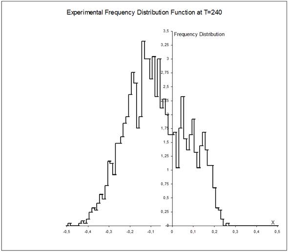
Fig. 1. Histogram of experimental frequency distribution function for a=10.at T=240.

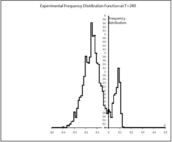
Fig. 2. Histogram of experimental frequency distribution function for a=30 at T=240.

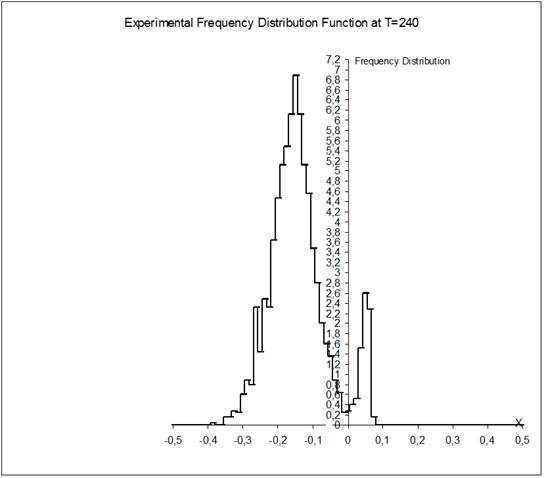
Fig. 3. Histogram of experimental frequency distribution function for a=60 at T=240.

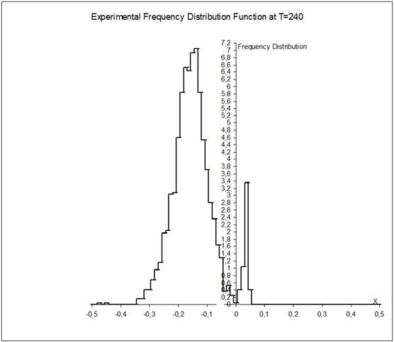
Fig. 4. Histogram of experimental frequency distribution function for a=100 at T=240.

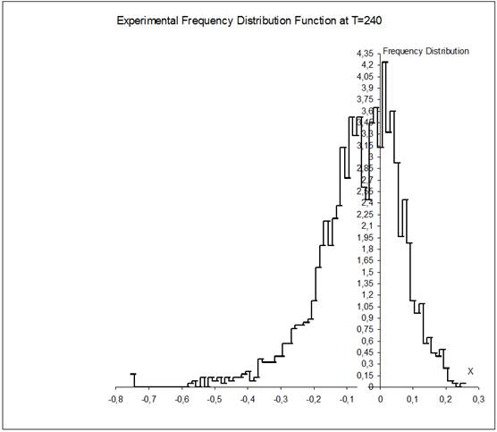
Fig. 5. Histogram of experimental frequency distribution function for a=60 at T=240.

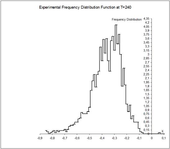
Fig. 6. Histogram of experimental frequency distribution function for a=60 at T=240.

4. Conclusions

As a result of number numerical experiments that simulate the Brownian walk particles along the plane exhibiting the spatial friction non-linearity characterizing by its increasing as x rises, we find that monotone increasing of the nonlinearity rate can lead to so large changes in the frequency distribution function graph shape that it looks like completely different from the one we observe usually. Namely, studying the frequency distribution function of the particles that walk randomly in homogeneous media we observe the one-top frequency distribution function while, in the non-homogeneous media with non-linear friction, the frequency distribution function graph can look like completely differently as a union of two such the one-top function graphs. In other words, the friction nonlinearity can lead to (and really result in) a bifurcation of the frequency distribution function. Bearing in mind that the pit associated with the frequency distribution function bifurcation arises and then continues to settle in the particle start point vicinity one can easily guess and make an infer of that the Brownian walk dynamics of the stochastic oscillators in non-linear non-homogeneous media depends very essentially on a point the ones start from. In doing so it can occur (and takes place, as we observed above, really) that the resulting dynamics will yield the distribution function whose density will have the deepest local minimum in the oscillator start point vicinity. In other words, a probability to encounter the oscillator in the given vicinity is small enough. It shows, in particular, that chaotic systems in non-linear non-homogeneous media can possess the very unusual interesting features.

References

1. Haken H. Synergetics. Springer. Berlin, 1983.
2. Haken H. Advanced synergetics. Springer. Berlin, 1985.
3. Zaslavsky G.M., Sagdeev R.Z., Usikov D.A. and Chernikov A.A. Weak chaos and quasi-regular patterns. Cambridge University Press. Cambridge, 1987.
4. Rěvěsz P. Random walk in random and non-random environments. World Scientific. Singapore, 1990.
5. Protter P. Stochastic integration and differential equations. Springer. Berlin, 1992.
6. Schuster H.G. Deterministic Chaos. Springer. 3^rd edition. Berlin, 1995.
7. Karatzas I. and Shreve S.E. Brownian motion and stochastic calculus, Springer. 2^nd edition. Berlin, 1996.
8. Vavrin D.M., Ryabov V.B., Sharapov S.A. and Ito H.M. Chaotic states of weakly and strongly nonlinear oscillators with quasiperiodic excitation. Phys. Rev E 53, 1996, pp. 103-114.
9. Rodrigues R. and Tuckwell H. Statistical properties of stochastic nonlinear dynamical models of single spiking newrons and newral networks. Phys. Rev E 54, 1996, pp. 5585-5590.
10. Lücking H. Pathological tremors: Deterministic chaos or nonlinear oscillators? Chaos 10(1), 2000, pp. 278-288.
11. Gus S.A. and Sviridov M.V. "Green" noise in quasi-stationary stochastic systems. Chaos 11(3), 2001, pp. 605-610.
12. Higham D. An algorithmic introduction to numerical simulation of stochastic differential equations. SIAM Review 43, 2001, pp. 525-546.
13. Wang X. Probabilistic decision making by slow reverberation in cortical circuits. Neuron 36, 2002, pp. 1-20.
14. Ivanov M.A, Dobrynskiy V.A. Random walk of oscillator on the plane with non-homogeneous friction. Int. INFA-ANS J. Problems Nonlinear Analysis in Engineering Systems", vol. 12, no. 1(15), 2006, pp. 101-116.
15. Ivanov M.A, Dobrynskiy V.A. Stochastic dynamics of oscillator drift in media with spatially non-homogeneous friction, J. Automation and Information Sci., vol. 40., no. 7, 2008, pp. 9-25.