Numerical Simulation of Turbulent Dam-Break Flow Using the Level Set Method

Ashraf Balabel^*

Mechanical Engineering Dept., Taif University, Taif, Hawiyya, Kingdom of Saudi Arabia

Abstract

The present paper introduces numerical simulations for one of the most challenging problems of two-phase flows; namely, the unsteady movements of dam break flow considering the turbulence effects. A novel numerical method is developed and validated for solving such complicated problem by solving the Reynolds-Averaged Navier Stokes equations over a regular and structured two-dimensional computational grid using the control volume approach. The standard k-e turbulence model is applied for predicting the turbulence characteristics of the dam break flow. The transient evolution of the dam free surface is predicted by the level set method. The effects of the geometrical parameters of the initial dam shape and the density ration of the two phases on the dam front movement and dam topological changes are investigated. The obtained results showed a faster movement of the dam front in the downstream direction by increasing the dam height and the density ratio. Moreover, the topological changes of the dam free surface in later evolutions are also predicted.

Keywords

Dam Break Problem, Level Set Method, Numerical Simulation, Turbulence Modeling, Two-Phase Flow

Received: May 26, 2015
Accepted: June 13, 2015
Published online: July 15, 2015

@ 2015 The Authors. Published by American Institute of Science. This Open Access article is under the CC BY-NC license. http://creativecommons.org/licenses/by-nc/4.0/

1. Introduction

Many of industrial and engineering applications encounter a large number of two phase flows; e.g. atomization of liquid jets [Lefebvre (1989)], droplet dynamics [Fuster, Agbaglah, Josserand, Popinet and Zaleski (2009)], bubble flow [Sato (1975)]and other multiphase flow systems [Kolev (2007)].

Dam break problem is considered to be one of the most important two-phase applications in engineering and industrial fields, e.g. hydropower stations, marine hydrodynamics and coastal engineering. Consequently, dam break flow has been the subject of extensive experimental, theoretical and numerical investigations for more than a hundred year. Detailed literature review for such problem can be found in [Park, JinKim, Van (2012)].

Experimental studies on dam break problem have observed the shape of the water propagation front and its traveling distance in the horizontal direction. In particular, the representative experimental investigation, which is considered as a benchmark test for dam break problem, is referred to [Martin and Moyce (1952)]. This experiment was later repeated using another experimental techniques by [Koshizuka and Oka (1984), Stansby, Chegini and Barnes (1998)].

According to the experimental complexity of such problem, exact measurements of the interface shape are not available; however, some measuring data such as the reduction of the water column height and the horizontal traveling distance of the water front can be applied for the validation of the numerical methods through the quantitative comparison of the obtained results.

Moreover, the theoretical as well as the numerical treatments of the dam break problem have encountered some constraints related to the nature of the problem as it includes a transient, non-uniform free surface flow with large spatial and temporal gradients. Moreover, turbulence characteristics should be considered with the moving wave front which is driven by gravity developed turbulence. Therefore, most of the previous numerical treatments of such problem are usually simulated by neglecting turbulent stresses or using various empirical assumptions about the parameters of turbulence. Recently, there is a trend to replace the previous attempts with direct numerical simulations, large eddy simulations and advance turbulence modeling, see for more details [Oezgoekmen, Iliescu, Fischer, Srinivasan, and Duan (2007), Park, JinKim, Van (2012)].

According to the huge development in the numerical simulation of turbulent two-phase flows with wide range of length scales, carefully executed simulations in such context can virtually replace experiments [Eggers (1997)]. In general, the numerical predictions of turbulent dam break dynamics have been limited in accuracy partly by the performance of three key elements, viz.: development of the computational algorithm, interface tracking methods, and turbulence prediction models [Balabel (2013)].

A variety of numerical methods have been recently developed and validated to two-phase turbulent flow. However, an efficient and complete numerical method is not available. An extended review of numerical techniques applied for turbulent two-phase flow including adv/disadvantages can be found in [Shinjo and Umemura (2010)]. More recently, the author has developed a new numerical method, known as Interfacial Marker Level Set Method (IMLS), for predicting the complete dynamics of turbulent two-phase flows. This numerical method is validated and its accuracy is estimated through the performing of a wide range of industrial and engineering applications [Balabel (2011-2012-2013)]. This method is also further applied in the present paper and shortly explained in the following sections.

2. Computational Method

The physical configuration of the dam break problem is illustrated in Fig. 1. The width and the length of the computational domain are H and L, respectively. At the initial state, the water depth and width are h_o and x_o, respectively. The water column has the properties; density of 1000 kg/m³ and viscosity of 1.0´10^-3 Ns/m², while the surrounding air phase has the density of 1.0 kg/m³ and viscosity of 1.5´10^-5 Ns/m². The computational domain is extended in x- and y- directions and the computational structured grids are considered to be of uniform size in both directions.

The governing equations for the transient two-dimensional, isothermal and incompressible turbulent two-phase flow are first described in the next section. An explanation of the level set formulation is given as well. Following, the numerical method adopted for solving the appropriate governing equations with the associated boundary conditions are also discussed.

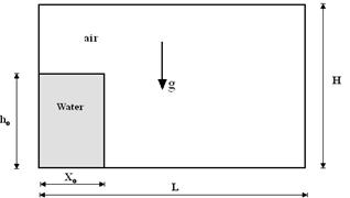
Figure 1. Computational domain of the dam break problem.

2.1. Reynolds-Averaged Navier-Stokes (RANS) Equations

The Reynolds form of the continuity and momentum equations for turbulent two-phase flow, called here RANS equations, at each point of the flow field including the gravitational field can be represented by the following equations:

                              (1)

    (2)

Where the subscript a takes the values 1 and 2 and refers to each phase properties, i.e., the liquid and gas (l, g) phases, respectively. In the above system of equations,  is the velocity vector, r is the density, p is the pressure, m is the molecular viscosity, is the strain rate tensor and is the turbulent stress tensor which are given as:

                              (3)

                 (4)

where  is the Kronecker delta and are the average of the velocity fluctuations. The turbulent viscosity is defined as:

                                      (5)

The turbulent kinetic energy k and its dissipation rate e can be estimated by solving the following equations:

  (6)

        (7)

The coefficients for the so-called STD k-e turbulence model are given as follows [Launder and Spalding (1974)]:

2.2. Boundary Conditions

Considering the computational domain, shown in figure 1, two kinds of boundary conditions are applied, the external domain and the interfacial boundary conditions. The numerical boundary conditions applied for external domain are based on the slip boundary conditions (u_i. n_i=0) for the bottom and sides of the computational domain, while zero stress boundary conditions are prescribed on the open upper boundary as explained by [Kaceniauskas (2008)]. The standard wall function for the turbulent boundary layer is employed so that both k and ε can be expressed as a function of the distance from the solid boundary and the shear velocity [Launder and Spalding (1974)].

In contrast to the previous two-phase boundary conditions [Brackbill, Lothe and Zemach (1992)], in which the surface tension effects are included in the momentum equations as an external body force, the present model sets the surface tension pressure explicitly in the interfacial boundary conditions formulation in the normal direction as:

                           (8)

In the present modelling, all the interfacial forces arising from the interfacial jump conditions are including in the pressure term in such a way:

                            (9)

The treatment of such terms in the adopted numerical algorithm can be seen in [Balabel (2012)]. The above system of equations and boundary conditions, Eqs.(1-9) are solved simultaneously to determine the topological changes of the free surface of the dam during its evolution. The level set method is applied for advection of the deformable interface as described in the following section.

2.3. Level Set Function

The level set method is a type of capturing methods where a defined phase function f, is smoothed over the entire computational domain. The level set function at any given point is taken as the signed normal distance from the interface with positive on the liquid phase (i.e. f>0), and negative on the gas phase (i.e. f<0). Consequently, the interface is implicitly defined as the zero level set of the level set function.

The transport equation of the level set function can be described by the following equation:

                                (10)

where is the velocity vector. The geometrical properties of the interface, (normal vectors and curvature), can be defined as:

                            (11)

The original work of level set method in two-phase numerical simulation is referred to [Sussman, Smereka and Osher (1994)]. A review of such works can be found in the cited review [Sethian and Smereka (2003)]. However, the application of the level set method in capturing the moving interfaces in turbulent flows is indeed very scarce.

2.4. IMLS Numerical Scheme

In the present paper, the so called Interfacial Marker Level Set method (IMSL) is applied for predicting the dam break problem in turbulent flow. This numerical method is developed and validated by the present author and applied for a wide range of industrial and engineering applications. More details about IMSL method can be found in [Balabel (2013)].

3. Validation

The physical phenomena, such as breaking wave, shockwaves, subcritical and supercritical flows, occurring in some cases of dam break problem includes it into the complex applications of free surface flows. The dam break problem introduces a great challenge of two-phase flow as it is a transient, non-uniform free surface flow with large spatial and temporal gradients [Yang, Lin, Jiang and Liu (2010)]. Moreover, including the turbulence in such case makes it much complex regarding its modeling from the numerical point of view. Recently, there are few attempts to simulate the dam break problem with LES as they allow a much deeper insight into the associated dynamics [Oezgoekmen, Iliescu, Fischer, Srinivasan and Duan (2007)].

In the present section, the present developed numerical method is validated by performing the dam break problem in turbulent regime and comparing the obtained numerical results with several sets of previous experimental measurements of [Stanby, Chegini, and Barnes (1998)] and the numerical results of [Shigematsu, Liu and Oda (2004)]. The dimensions of the considered problem are (L=2m, H=0.25m, h_o=0.1m and X_o=1m).

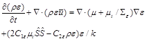
Figure 2 shows the comparison of the obtained numerical results for the dimensionless displacement of the dam break in turbulent flow The dimensionless time and displacement are given by and x*=x/h_o. First, a grid independent study is carried out using different grid resolutions. It can be shown that, starting from 200x50 grid points in x- and y-directions, the present numerical results are in better agreement with the experimental measurements than the previous numerical results of [Shigematsu, Liu and Oda (2004)].

4. Results and Discussion

Figure 3 illustrates the transient free surface evolution of the breaking dam along with the predicted turbulent kinetic energy distribution at different time instants. It can be noticed that, during the wave propagation of the dam break, turbulence is generated and it concentrates near the moving wave front. In general, it can be concluded that, the present numerical method can successfully predict the complex topological changes of the dam break problem in turbulent flow.

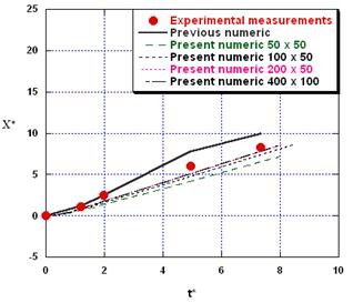
Figure 2. Comparison of the obtained numerical results for dimensionless horizontal displacement of dam break with experimental measurements of (Stanby et al., 1998), and the previous numerical results of (Shigematsu et al., 2004).

Figure 3. The transient free surface of the dam break along with the predicted turbulent kinetic energy, k (m²/s²), at different dimensionless times.

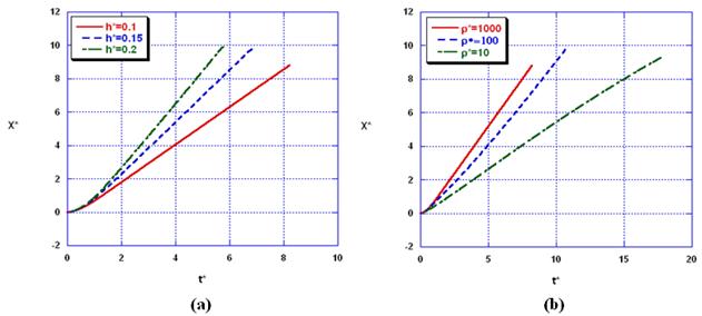
Figure 4. The Effect of dam height (a) and density ratio (b) on the downstream movement of dam front.

4.1. The Effect of Dam Height and Density Ratio on Dam Break

Figure 4 (a, b) shows the effects of dam height h*=h_o/X_o and the density ratio r*=r_water/r_air on the downstream movement of the dam front. As shown in the figure, the increasing of the dam height leads to a fast movement of the dam front that can reach to the other side of the computational domain in short time. The same effect can be also observed by increasing the density ratio of the two phases.

4.2. Prediction of Dam Free Surface at Later Evolutions

Figure 5 shows the topological changes of the dam free surface at later time of breaking for h*=0.2 and density ratio of 1000. It is clear that the present numerical method can successfully capture the complex topological changes of the turbulent free surface during the dam breaking. The formation of an entrapped air cavity is clearly visible. The treatment of such cavity during the numerical simulation is carried out in normal way without any numerical ad-hoc assumptions.

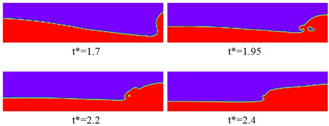
Figure 5. The topological changes of dam break at later times.

5. Conclusion

In the present paper, the dam break problem in turbulent field is numerically simulated. The numerical method is based on solving the RANS equations with a developed numerical method known as IMLS method. The tracking and capturing of the dam free surface is carried out by the level set method. The comparison of the obtained numerical results showed a good agreement with the previous experimental measurements better than previous numerical results from the previous publications. Generally, it can be concluded that the implementation of the developed numerical method in three dimensional two-phase turbulent applications can be straightforward and the extension of the numerical model to include a wide range of industrial and engineering applications could be easily task.

References

1. Lefebvre, A. H.(1989): Atomization and sprays, Hemisphere Publishing Corporation.
2. Fuster, D., Agbaglah, G., Josserand, C., Popinet, S. and Zaleski, S.(2009): Numerical simulation of droplets, bubbles and waves: state of the art, Fluid Dyn. Res. 41, 1-24.
3. Sato, Y.(1975): Liquid velocity distribution in two phase bubble flow, Int. J. Multiphase flow, vol. 2(1), pp. 79-95.
4. Kolev N.I., (2007): Multiphase flow dynamics: Thermal and Mechanical Interaction", Springer.
5. Park, R., JinKim, K., Van, S.(2012): Numerical investigation of the effects of turbulence intensity on dam-break flows,Ocean Engineering, vol. 42, pp. 176–187.
6. Martin, J. C. and Moyce, W. J., (1952): An Experimental Study of the Collapse of a Liquid Column on a Rigid Horizontal Plane,Phil. Trans. Royal Soc. London A244, pp. 312-324.
7. Koshizuka, S., Oka, Y.,(1984): Moving particle semi-implicit method for fragmenta- tion of incompressible fluid. Nucl. Sci. Eng. vol. 123, pp. 421–434.
8. Stansby, P.K., Chegini, A., Barnes, T.C.D.,(1998): The initial stages of dam-break flow. J. Fluid Mech. 374, 407–424.
9. Oezgoekmen, T. M., Iliescu, T., Fischer, P.F., Srinivasan, A. and Duan, J.,(2007): Large eddy simulation of stratified mixing and two-dimensional dam break problem in a rectagular enclosed domain. Ocean Modelling, vol. 16, pp.106–140.
10. Eggers, J. (1997): Nonlinear Dynamics and Breakup of Free-Surface Flow, Rews. Modern Phys., vol. 69, No. 3, pp. 865–929.
11. Balabel A. (2013):Numerical Modelling of Liquid Jet Breakup by Different Liquid Jet/Air Flow Orientations Using the Level Set Method, Computer modeling in engineering & sciences, vol. 95 (4), pp. 283-302.
12. Shinjo J. and Umemura A.,(2010): Simulation of liquid primary breakup: Dynamics of ligament and droplet formation", Int. J. Multiphase Flow, vol. 36(7), pp. 513-532.
13. Balabel, A.; El-Askary, W.(2011): On the performance of linear and nonlinear k–e turbulence models in various jet flow applications. European Journal of Mechanics B/Fluids, vol. 30, pp. 325–340.
14. Balabel, A.(2011): Numerical prediction of droplet dynamics in turbulent flow, using the level set method. International Journal of Computational Fluid Dynamics, vol. 25, no. 5, pp. 239-253.
15. Balabel, A.(2012): Numerical simulation of two-dimensional binary droplets collision outcomes using the level set method. International Journal of Computational Fluid Dynamics, vol. 26, no. 1, pp. 1-21.
16. Balabel, A.(2012): Numerical modeling of turbulence-induced interfacial instability in two-phase flow with moving interface. Applied Mathematical Modelling, vol. 36, pp. 3593–3611.
17. Balabel, A.(2012): A Generalized Level Set-Navier Stokes Numerical Method for Predicting Thermo-Fluid Dynamics of Turbulent Free Surface. Computer Modeling in Engineering and Sciences (CMES), vol.83, no.6, pp. 599-638.
18. Balabel, A.(2012): Numerical Modelling of Turbulence Effects on Droplet Collision Dynamics using the Level Set Method. Computer Modeling in Engineering and Sciences (CMES), vol. 89, no.4, pp. 283-301.
19. Balabel, A, El-askary, W., Wilson, S.(2013):Numerical and Experimental Investigations of JetImpingement on a Periodically Oscillating-Heated FlatPlate. Computer Modeling in Engineering and Sciences (CMES), vol. 95 (6), pp. 483-499.
20. Launder, B. E., Spalding, D. B.(1974): The numerical computation of turbulent flow, Computer Methods in Applied Mechanics and Engineering, vol. 3(2), pp. 269-289.
21. Kaceniauskas, A.(2008): Development of efficient interface sharpening procedure for viscous incompressible flows, INFORMATICA, vol. 19(4), pp. 487-504.
22. Brackbill, J. U., Kothe, D. B. and Zemach. A.(1992). A Continuum Method for Modeling Surface Tension, J. Comp. Physics, 100, 335-354.
23. Sussman, M., Smereka, P. and Osher, S.(1994): A level set approach for computing solutions to incompressible two-phase flows, J. Comp. Physics, 114, 146-159.
24. Balabel, A.(2013): Numerical Modelling of Liquid Jet Breakup by Different Liquid Jet/Air Flow Orientations Using the Level Set Method. Computer Modeling in Engineering and Sciences (CMES), vol. 95, no.4, pp. 283-302.
25. Yang, C., Lin, B., Jiang, C. And Liu, Y. (2010):Predicting near-field dam-break flow and impact force using a 3D model, J. Hydr. Research, vol. 48 (6), pp. 784-792.
26. Oezgoekmen, T. M., Iliescu, T., Fischer, P.F., Srinivasan, A. and Duan, J., (2007):Large eddy simulation of stratified mixing and two-dimensional dam break problem in a rectagular enclosed domain. Ocean Modelling, vol. 16, pp. 106–140.
27. Stanby, P.K., Chegini, A. and Barnes, T.C.D. (1998): The Initial Stage of Dam-break Flow." J. Fluid Mech. vol. 374, pp. 407–424.
28. Shigematsu, T., Liu, P., and Oda, K. (2004):Numerical modeling of the initial stages of dam-break waves, J. of Hydr. Research, vol. 42 (2), pp. 183–195.