
Journal of Nanoscience and Nanoengineering, Vol. 1, No. 4, December 2015 Publish Date: Sep. 13, 2015 Pages: 183-192
MHD Stagnation-Point Flow and Heat Transfer of Nanofluid over a Shrinking Surface
Samir Kumar Nandy1, *, Rajib Kumar Mandal2
1Department of Mathematics, A.K.P.C Mahavidyalaya, Bengai, Hooghly, India
2Department of Physics, A.K.P.C Mahavidyalaya, Bengai, Hooghly, India
Abstract
This paper analyzes the combined effects of magnetic field, Brownian motion, thermophoresis and thermal radiation on stagnation–point flow and heat transfer due to nanofluid towards a nonlinearly stretching/shrinking sheet. A variable magnetic field is applied normal to the sheet. Using a similarity transformation, the governing mathematical equations are transformed into coupled nonlinear ordinary differential equations which are then solved numerically using fourth order Runga–Kutta method with shooting technique. Different from a nonlinearly stretching sheet, it is found that the solutions for a nonlinearly shrinking sheet are non-unique. The numerical results pertaining to the present study indicate that the magnetic field parameter enhances the existence range of solution domain. The influences of various relevant parameters on flow, temperature and concentration as well as skin friction coefficient, local Nusselt number and local Sherwood number are investigated. A comparison with the previous study available in the literature is done and we found an excellent agreement with them.
Keywords
Stagnation-Point Flow, Heat Transfer, Nanofluid, Magnetic Field, Thermal Radiation
Received: August 3, 2015
Accepted: August 26, 2015
Published online: September 13, 2015
@ 2015 The Authors. Published by American Institute of Science. This Open Access article is under the CC BY-NC license. http://creativecommons.org/licenses/by-nc/4.0/
1. Introduction
One of the methods for enhancing heat transfer is the application of additives to the working fluid. The basic idea is to enhance heat transfer by changing the fluid transport properties such as in nanofluid, where solid particles are added to the base fluid to increase its thermal conductivity. Nanofluid consists of a base fluid such as water and nanocell metallic or non metallic particles. The term nanofluid was first used by Choi [1] to indicate engineered colloids composed of nanoparticles dispersed in a base fluid. Then using a nanofluid as a heat transfer working fluid has gained much attention in recent years due to its potential advantages which include higher thermal conductivity than the pure fluids, excellent stability and little increase in pressure drop. Due to better performance of heat exchange, the nanofluids can be utilized in several engineering and industrial applications which include power generation in a power plant, production of micro electronics, advanced nuclear system and many others. Because of the wide range of applications of nanofluids, significant research interest has been carried out in recent years to study heat transfer characteristics of such fluids.
Nanofluid is actually a homogeneous mixture of base fluid and nanoparticles. Nanofluid is a fluid contains nanometer sized particles, called nanoparticles. These fluids are engineered colloidal suspensions of nanoparticles in a base fluid. Some nanoparticle materials that have been used in nanofluids are Oxide Ceramics (Al2O3, CuO), Nitride Ceramics (AlN, SiN), Carbide Ceramics (SiC, TiC), metals (Ag, Au, Cu, Fe), semiconductors (TiO2) and single, double or multi-walled carbon nanotubes (SWCNT, DWCNT, MWCNT). The base fluid is usually a conductive fluid, such as water, ethylene glycol, oil and other lubricants and polymer solutions. Normally the size of the nanoparticle is1–100 nm in diameter but according to shape and size, it can vary slightly. In addition, few commonly used base fluids namely water, engine oil or ethylene glycol have poor thermal conductivity. To enhance the thermal conductivity of such kind of base fluids, nanoparticles are suspended in the fluids so that the thermal conductivity of the mixture (nanofluid) can be enhanced ultimately. Nanofluids commonly contain up to a 5 % volume fraction of nanoparticles to ensure effective heat transfer enhancement (see [2], [3]).
The study of stagnation point flow and heat transfer over a stretching surface has a large number of applications such as in the colons of electronic devices, paper production, glass blowing and continuous casting, aerodynamic extrusion of plastic sheets, etc. On the other hand, the flow of an electrically conducting fluid over a stretching surface in the presence of a transverse magnetic field has attracted the attention of many researchers in view ofits wide applications in many industrial problems such as MHD generators, nuclear reactors, geothermal energy extraction and boundary layer flow control in the field of aerodynamics. Different aspects of the flow and heat transfer over a continuous moving surface have been investigated by different researchers under different physical conditions (see [4]-[10]).
Meanwhile, after the pioneering work of Choi [1], studies related to the nanofluid dynamics have increased greatly in recent due to its wide applications in both industrial and engineering systems. A comprehensive review of the literature about nanofluids is given in the references [11]-[12]. The Cheng-Minkowycz problem for flow of nanofluid embedded in a porous medium was considered by Nield and Kuznetsov [13]. Natural connective boundary layer flow of nanofluid past a vertical flat plate was studied by Kuznetsov and Nield [14]. Bachok et al [15] investigated the flow of nanofluid over a continuously moving surface with a parallel free stream. Khan and Pop [16] investigated the boundary layer flow of nanofluid past a linear stretching sheet. Yacob et al [17] solved the Falkner–Skan problem for flow of nanofluid with prescribed surface heat flux. In a recent paper, Makinde and Aziz [18] discussed the effect of convective boundary conditions on the flow of nanofluid past a stretching sheet. Recently Ibrahim et al [19] numerically analyzed the hydromagnetic stagnation point flow and heat transfer due to nanofluid towards a stretching sheet.
Recently, the flow over a shrinking sheet has attracted the attention of many researchers. In this type of flow, the fluid is stretched towards a slot and the flow is quite different from the stretching case. The physical reason is that the vorticity generated due to shrinking sheet is not confined within the boundary layer and consequently a situation appears where some other external forces are to be imposed. In confining the vorticity within the boundary layer, the external forces are either suction at the sheet (Miklavcic and Wang [20]) or stagnation flow added to main flow (Wang [21]). Later several researchers studied the boundary layer flow over a shrinking surface under different physical conditions ([22]-[25]).
All studies mentioned above refer to the boundary layer flow towards a stretching/shrinking sheet in a viscous Newtonian fluid. Meanwhile, stagnation point flow and mass transfer with chemical reaction past a permeable stretching/shrinking sheet in a nanofluid was studied by Rosca et al [26]. Unsteady boundary layer flow and heat transfer of nanofluid over a permeable stretching/shrinking sheet was investigated by Bachok et al [27] and they found that dual solutions exist for shrinking sheet. In another paper, the unsteady flow over a continuously shrinking surface with wall mass suction in a nanofluid was investigated by Rohni et al [28]. Very recently the effects of slip and heat generation/absorption on MHD boundary layer stagnation point flow and heat transfer of nanofluid over a stretching / shrinking surface was analyzed by Nandy and Mahapatra [29].
The objective of the present study is to investigate the dynamics of the natural convection boundary layer stagnation point flow and heat transfer of a viscous incompressible nanofluid over a nonlinearly shrinking surface in the presence of an applied magnetic field and thermal radiation. In certain polymeric and metallurgical processes, nonlinearly stretching /shrinking effects are very much important because the final product is strongly influenced by the processes of stretching and the rate of cooling. Thus the main focus of the analysis is to investigate how flow and temperature fields of a nanofluid influenced by the magnetic parameter, the nonlinearity of the sheet and the thermal radiation. To the best of our knowledge, no research has been carried out considering the above stated flow model for a nanofluid.
2. Flow Analysis
We consider the steady two dimensional stagnation-point flow of a viscous incompressible nanofluid over a nonlinearly stretching/shrinking sheet in the presence of magnetic field and thermal radiation. The coordinates (x,y) are such that x is along the sheet and y is normal to the sheet. A variable magnetic field of strength B(x) is applied in a direction normal to the sheet. It is assumed that the velocity of the sheet is uw(x) =cxnwhere c is a dimensional constant, known as the stretching / shrinking rate and n is an arbitrary positive constant known as the stretching index. The velocity outside the boundary layer is u(x)=axn, where a >0 is a constant denotes the strength of the stagnation flow. We also assume that the constant temperature and constant nanoparticle fraction at the surface of the sheet are Tw and Cw, while these values in the ambient fluid are denoted by T∞ and C∞, respectively. A schematic representation of this problem is shown in Fig.1.
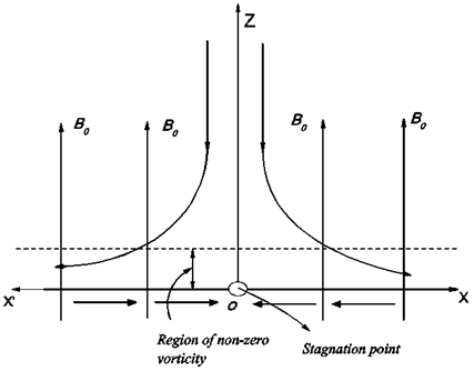
Fig. 1. Physical model and the coordinate system.
Under these assumptions, the basic conservation equations of mass, momentum, thermal energy and nanoparticle fraction can be written as
![]() (1)
(1)
![]()
![]() ν
ν![]()
![]() (2)
(2)
 (3)
(3)
![]()
![]() (4)
(4)
The velocity components along x and y axes are u and v respectively, υ is the kinematics viscosity, σ is the electrical conductivity, ρ is the density, cp is the specific heat at constant pressure, αm is the thermal diffusivity, DB is the Brownian diffusion coefficient, DT is the thermophoresis coefficient, qr is the radiative heat flux, τ is the ratio between the effective heat capacity of the nanoparticle material and heat capacity of the fluid and U(x) is the free stream velocity.
The term ![]() in the R.H.S of equation (2) is the Lorentz force which arises due to the interaction of the fluid velocity and the applied magnetic field. In writing equation (2), we have neglected the induced magnetic field since the magnetic Reynolds number for the flow is assumed to be very small. This assumption is justified for flow of electrically conductive fluids such as liquid metals e.g. mercury, liquid sodium etc. (see Shercliff [30]). Also for similarity solution, we assume that the transverse magnetic field strength applied to the sheet is
in the R.H.S of equation (2) is the Lorentz force which arises due to the interaction of the fluid velocity and the applied magnetic field. In writing equation (2), we have neglected the induced magnetic field since the magnetic Reynolds number for the flow is assumed to be very small. This assumption is justified for flow of electrically conductive fluids such as liquid metals e.g. mercury, liquid sodium etc. (see Shercliff [30]). Also for similarity solution, we assume that the transverse magnetic field strength applied to the sheet is ![]() , where B0 is the constant magnetic field.
, where B0 is the constant magnetic field.
Equation (3) depicts that heat can be transported in a nanofluid by convection, by conduction and also by virtue of nanoparticle diffusion and radiation. The term ![]() is the heat convection, the term
is the heat convection, the term ![]() is the heat conduction; the term
is the heat conduction; the term ![]() is the thermal energy transport due to Brownian diffusion, the term τ
is the thermal energy transport due to Brownian diffusion, the term τ![]() is the energy transport due to thermophoretic effect and
is the energy transport due to thermophoretic effect and ![]() is the nanoparticle heat diffusion by radiation.
is the nanoparticle heat diffusion by radiation.
Equation (4) shows that the nanoparticles can move homogeneously within the fluid (by the term ![]() ), but they also possess a slip velocity relative to the fluid due to Brownian diffusion
), but they also possess a slip velocity relative to the fluid due to Brownian diffusion ![]() and the thermophoresis
and the thermophoresis![]() .
.
The boundary conditions for the present problem are
u = Uw(x)=cxn, ν=0, T=Tw , C=Cw, at y=0
u→U(x) = axn ,T→ T∞ ,C→![]() as y→∞ (5)
as y→∞ (5)
The radiative heat flux (Sparrow and Cess [31] or Magyari and Pantokratoras [32]) is given as
![]() = -
= -![]() (6)
(6)
where![]() (=
(= ![]() ) is the Stefan Boltzmann constant and
) is the Stefan Boltzmann constant and ![]()
![]() is the Rosseland mean absorption coefficient. Assuming the temperature difference within the flow is such that
is the Rosseland mean absorption coefficient. Assuming the temperature difference within the flow is such that ![]() can be expanded in a Taylor series about
can be expanded in a Taylor series about ![]() and neglecting higher order terms, we get
and neglecting higher order terms, we get ![]() .
.
Hence from equation (6) and using the above result, we have
![]()
![]() (7)
(7)
We look for a similarity solution of equations (2)-(4) together with the boundary conditions (5) of the following form
 (8)
(8)
where the stream function ψ is defined in the usual way as
![]()
Hence from equation (8) we have
![]() ,
,
![]() (9)
(9)
Substituting equations (8) and (9) into equations (2) – (4), we have the following ordinary differential equations as
![]() (10)
(10)
![]() (11)
(11)
![]() (12)
(12)
where the prime denotes the differentiation with respect to the similarity variable η. The dimensionless parameters for this problem are ![]() is the magnetic parameter,
is the magnetic parameter, ![]() is the effective Prandtl number, R
is the effective Prandtl number, R ![]() is the radiation parameter,
is the radiation parameter,![]() is the Prandtl number, Nb
is the Prandtl number, Nb![]() is the Brownian motion parameter, Nt
is the Brownian motion parameter, Nt![]() is the thermophoresis parameter and
is the thermophoresis parameter and![]() is the Lewis number.
is the Lewis number.
The boundary conditions then become
 (13)
(13)
Quantities of physical interest are the skin friction coefficient ![]() , the local Nusselt number
, the local Nusselt number ![]() and the local Sherwood number
and the local Sherwood number ![]() , which are defined as
, which are defined as
![]() (14)
(14)
where ![]() is the surface shear stress,
is the surface shear stress, ![]() is the surface heat flux and
is the surface heat flux and ![]() is the mass flux at the surface, which can be expressed as
is the mass flux at the surface, which can be expressed as
![]()
![]()
![]() (15)
(15)
Hence using(8) and (15) in equation (14), we have
![]() ,
,![]() ,
,
![]() (16)
(16)
where![]() is the local Reynolds number.
is the local Reynolds number.
3. Numerical Method
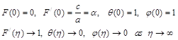
Numerical solutions to the governing non-linear ordinary differential equations (10)–(12) subject to the boundary conditions (13) have been solved numerically for different values of the governing parameters using fourth order Runge–Kutta scheme coupled with a conventional shooting procedure. In this method, dual solutions are obtained by setting different initial guesses for the values of F''(0), -θ'(0) and -φ'(0) where all profiles satisfy the far field boundary conditions asymptotically but with different shapes. Step size of Δη = 0.001 and the convergence criteria![]() are used in the program. In practice η =∞ must be replaced by an approximation η = η max , where η max is arbitrary as long as chosen large enough. We ran our computations with the value ηmax=12, which was sufficient to achieve the far field boundary conditions asymptotically for all values of the parameters considered.
are used in the program. In practice η =∞ must be replaced by an approximation η = η max , where η max is arbitrary as long as chosen large enough. We ran our computations with the value ηmax=12, which was sufficient to achieve the far field boundary conditions asymptotically for all values of the parameters considered.
4. Verification of the Computer Code
To verify our computer code, we check the results in terms of skin friction coefficient F''(0) for different values of α (< 0) with those of Bhattacharyya [24] and Rosca et al [26] in the absence of some particular parameters. The comparison given in Table 1 shows excellent agreement between the results and gives us confidence in our numerical approach.
Table 1. Comparison of the values of F''(0)with M=0, n=1 for viscous fluid with those of Bhattacharyya [24] and Rosca et al [26] for several values ofα (< 0).
| Present study | Bhattacharyya [24] | Rosca et al[26 ] | ||||
| 1st soln. | 2nd. soln | 1st soln. | 2nd. soln | 1st soln. | 2nd. soln | |
| -0.25 | 1.402242 | 1.4022405 | 1.4022407 | |||
| -0.50 | 1.495672 | 1.4956697 | 1.4956697 | |||
| -0.75 | 1.489296 | 1.4892981 | 1.4892981 | |||
| -1.0 | 1.328819 | 0 | 1.3288169 | 0 | 1.3288168 | 0 |
| -1.15 | 1.082232 | 0.116702 | 1.0822316 | 0.1167023 | 1.0822311 | 0.1167020 |
| -1.20 | 0.932470 | 0.233648 | 0.9324728 | 0.2336491 | 0.9324733 | 0.2336496 |
| -1.2465 | 0.584374 | 0.554208 | 0.5842915 | 0.5542856 | 0.5842816 | 0.5542962 |
5. Results and Discussion
The influence of the magnetic field on the wall shear stress ![]() is shown in Fig. 2. The shear stress acting between the wall and fluid layer is defined as the wall shear stress. It is observed that the solution for particular values of M exists up to a critical value
is shown in Fig. 2. The shear stress acting between the wall and fluid layer is defined as the wall shear stress. It is observed that the solution for particular values of M exists up to a critical value![]() (say), beyond which the boundary layer separates from the sheet and the solution based on the boundary layer approximations is not possible. The solution is unique for
(say), beyond which the boundary layer separates from the sheet and the solution based on the boundary layer approximations is not possible. The solution is unique for![]() (i.e., for stretching sheet) and non-unique for
(i.e., for stretching sheet) and non-unique for![]() (i.e., for shrinking sheet). From numerical computations, we have found that for M= 0.0, the critical values of
(i.e., for shrinking sheet). From numerical computations, we have found that for M= 0.0, the critical values of ![]() (which is
(which is ![]() ) = -1.278104, for M =0.1,
) = -1.278104, for M =0.1, ![]() -1.353544and for M = 0.2,
-1.353544and for M = 0.2, ![]() -1.429454. From the figure it is observed that the values of F' '(0) increases as |α| increases and these values reach the maximum before decreasing to zero. The maximum value is higher if the effect of magnetic field is strong. This is due to the fact that application of a magnetic field to an electrically conducting fluid produces a drag-like force called Lorentz force. Hence this Lorentz force will be enhanced by increasing M, which imparts additional momentum into the boundary layer. Also the application of the magnetic field enhances the existence range of solution domain. The variation of heat transfer rate -θ'(0) and concentration rate - φ’(0) with α for different M are shown in Figs. 3 and 4. From these figures, we can conclude that due to an increment of the values of M, both heat transfer rate and concentration rate increase. These figures also reveal the existence of dual solutions for both heat transfer rate and concentration rate.
-1.429454. From the figure it is observed that the values of F' '(0) increases as |α| increases and these values reach the maximum before decreasing to zero. The maximum value is higher if the effect of magnetic field is strong. This is due to the fact that application of a magnetic field to an electrically conducting fluid produces a drag-like force called Lorentz force. Hence this Lorentz force will be enhanced by increasing M, which imparts additional momentum into the boundary layer. Also the application of the magnetic field enhances the existence range of solution domain. The variation of heat transfer rate -θ'(0) and concentration rate - φ’(0) with α for different M are shown in Figs. 3 and 4. From these figures, we can conclude that due to an increment of the values of M, both heat transfer rate and concentration rate increase. These figures also reveal the existence of dual solutions for both heat transfer rate and concentration rate.
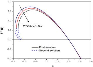
Fig. 2. Variation of the skin friction coefficient ![]() with
with ![]() for different values of the magnetic parameter M with n=1.2.
for different values of the magnetic parameter M with n=1.2.
Fig. 3. Variation of the Nusselt number ![]() with
with ![]() for different values of the magnetic parameter M with Nb=Nt=0.1, Le=1, Pr=0.71, Preff=0.5 and n=1.2.
for different values of the magnetic parameter M with Nb=Nt=0.1, Le=1, Pr=0.71, Preff=0.5 and n=1.2.
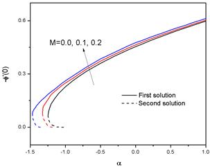
Fig. 4. Variation of the Sherwood number ![]() with
with ![]() for different values of the magnetic parameter M with Nb=Nt=0.1, Le=1, Pr=0.71, Preff=0.5 and n=1.2.
for different values of the magnetic parameter M with Nb=Nt=0.1, Le=1, Pr=0.71, Preff=0.5 and n=1.2.
Figures 5-7 represent the horizontal velocity component ![]() the temperature θ(η) and the nanoparticle concentration φ(η) for different values of the magnetic parameter M with fixed values of the other parameters. Fig. 5 depicts the dual velocity profiles
the temperature θ(η) and the nanoparticle concentration φ(η) for different values of the magnetic parameter M with fixed values of the other parameters. Fig. 5 depicts the dual velocity profiles ![]() for several values of M. The figure also reveals that the velocity at a point increases with increase in M for the first solution and the reverse is true for the second solution. The first solution approaches to unity (since
for several values of M. The figure also reveals that the velocity at a point increases with increase in M for the first solution and the reverse is true for the second solution. The first solution approaches to unity (since ![]() ) faster than the second solution, which is consistent with the fact that the boundary layer thickness of the first solution is smaller than that of the second solution. Figs 6 & 7 show temperature profiles θ(η) and concentration profiles φ(η) versus η for different values of M. From these figures, we found that the temperature and the concentration of a nanofluid both decrease with the increase of M (for first solution). This is due to the fact that the application of a magnetic field on the flow domain creates a Lorentz force which accelerates the fluid motion and as a consequence the temperature of the fluid within the boundary layer decreases. The thickness of the thermal boundary layer also decreases with the increase of M. Thus the surface temperature and nanoparticle concentration of the sheet can be controlled by controlling the strength of the applied magnetic field.
) faster than the second solution, which is consistent with the fact that the boundary layer thickness of the first solution is smaller than that of the second solution. Figs 6 & 7 show temperature profiles θ(η) and concentration profiles φ(η) versus η for different values of M. From these figures, we found that the temperature and the concentration of a nanofluid both decrease with the increase of M (for first solution). This is due to the fact that the application of a magnetic field on the flow domain creates a Lorentz force which accelerates the fluid motion and as a consequence the temperature of the fluid within the boundary layer decreases. The thickness of the thermal boundary layer also decreases with the increase of M. Thus the surface temperature and nanoparticle concentration of the sheet can be controlled by controlling the strength of the applied magnetic field.
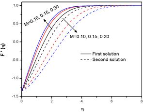
Fig. 5. Variation of the velocity profiles ![]() for several Values of M with α =-1.35 and n=1.2.
for several Values of M with α =-1.35 and n=1.2.
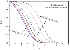
Fig. 6. Variation of the temperature distribution ![]() for several values of M with α = -1.35, Nb = Nt = 0.1, Le = 1, Preff =0.7 and n=1.2.
for several values of M with α = -1.35, Nb = Nt = 0.1, Le = 1, Preff =0.7 and n=1.2.
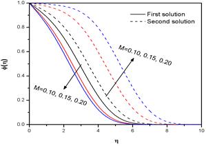
Fig. 7. Variation of the concentration profiles φ(η) for several values of M with α =-1.35, Nb = Nt = 0.1, Le = 1, Preff =0.7 and n=1.2.
Plots of the velocity profile ![]() for different values of α(< 0) for selected values of the other parameters are shown in Fig. 8. As |α |increases, the velocity of the fluid within the boundary layer also increases for the first solution. Fig. 9 depicts the variations of velocity profiles
for different values of α(< 0) for selected values of the other parameters are shown in Fig. 8. As |α |increases, the velocity of the fluid within the boundary layer also increases for the first solution. Fig. 9 depicts the variations of velocity profiles ![]() for different values of the stretching index parameter n. It is worth noting that a positive value of n corresponds to accelerated stretching surface whereas negative value of n corresponds to a decelerated stretching surface. The value n=0 represents a uniformly moving surface. In the present paper we have considered non negative values of n only. It is observed that nanofluid velocity increases with the increase of the non linearity stretching index n for the first solution and the flow velocity decreases with the increase of n for the second solution. The thickness of the hydrodynamic boundary layer increases with the increase of n.
for different values of the stretching index parameter n. It is worth noting that a positive value of n corresponds to accelerated stretching surface whereas negative value of n corresponds to a decelerated stretching surface. The value n=0 represents a uniformly moving surface. In the present paper we have considered non negative values of n only. It is observed that nanofluid velocity increases with the increase of the non linearity stretching index n for the first solution and the flow velocity decreases with the increase of n for the second solution. The thickness of the hydrodynamic boundary layer increases with the increase of n.
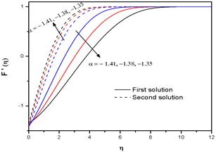
Fig. 8. Variation of the velocity profiles ![]() for several values of α(<0) with M=0.2 and n=0.8.
for several values of α(<0) with M=0.2 and n=0.8.
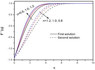
Fig. 9. Variation of the velocity profiles ![]() for several values of the power-law index parameter n with α =-1.40 and M=0.2.
for several values of the power-law index parameter n with α =-1.40 and M=0.2.
Fig. 10 shows the influence of the effective Prandtl number (Preff.) on the temperature profiles θ(η) for other fixed parameters. It is worth noting that Preff (=Pr/(1+4R/3) is nothing but a simple rescaling of the Prandtl number (Pr) by a factor involving the radiation parameter (R). So Preff is directly proportional to Pr and inversely proportional to R. Fig. 10 reveals that as Preff increases, the temperature at a point decreases except in a small region near the sheet (for first solution branch). Physically this can be explained as follows. An increase in Prandtl number (Pr) means a decrease of fluid thermal conductivity which ceases the reduction of the thermal boundary thickness. The second solution branch is different; for the given parameters as Preff increases temperature at a point also increases.
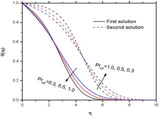
Fig. 10. Variation of the temperature distribution ![]() for several values of effective Prandtl number with α =-1.40, Nb = 0.1, Nt = 0.1, Le = 1, n=1.2 and M = 0.2.
for several values of effective Prandtl number with α =-1.40, Nb = 0.1, Nt = 0.1, Le = 1, n=1.2 and M = 0.2.
The influence of Brownian motion parameter (Nb) on dimensionless temperature θ(η) for the fixed values of other parameters is shown in Fig.11. The figure reveals that the dimensionless temperature within the boundary layer increases with increasing values of Nb for the first solution and decreases with increasing values of Nb for the second solution. The physical reason is that the Brownian motion enhances the thermal conduction due either to nanoparticle transporting heat or the micro-convection of the fluid surrounding individual nanoparticle. Fig. 12 represents the variation of thermophoresis parameter (Nt) on temperature profiles θ(η). It is seen from the figure that the thermophoresis parameter increases the temperature of the fluid for the first solution, but opposite behaviour is observed for the second solution. The variation of the concentration profiles φ(η) for different values of Lewis number (Le) is displayed in Fig 13. The figure reveals that for both the solution branches, up to a certain region φ(η) increases with the increase in the values of Le, but beyond this region φ(η) decreases with an increase in Le. It is to be noted that Lewis number (Le) is the ratio of thermal diffusivity to mass diffusivity and is generally used to characterize fluid flows where simultaneous heat transfer and mass transfer occur.
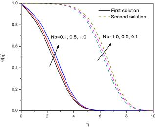
Fig. 11. Variation of the temperature distribution ![]() for several values of Nb with α = -1.40, Nt = 0.1, Le = 1, Preff =0.7, n=1.2 and M = 0.2.
for several values of Nb with α = -1.40, Nt = 0.1, Le = 1, Preff =0.7, n=1.2 and M = 0.2.
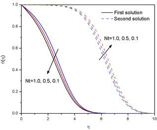
Fig. 12. Variation of the temperature distribution ![]() for several values of Nt with α = -1.40, Nb = 0.1, Le = 1, Preff =0.7, n=1.2 and M = 0.2.
for several values of Nt with α = -1.40, Nb = 0.1, Le = 1, Preff =0.7, n=1.2 and M = 0.2.
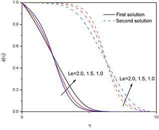
Fig. 13. Variation of the concentration profiles φ(η) for several values of Le with α = -1.40, Nb = Nt = 0.1, Preff =0.7, n=1.2 and M = 0.2.
6. Concluding Remark
In summary, the problem of MHD stagnation-point flow and heat transfer in a nanofluid past a nonlinearly stretching/shrinking sheet is studied in this paper. Similarity transformation technique is employed to reach the partial differential equations in to an ordinary differential equation group. The equation group is solved numerically using the shooting method. We have found that non–unique solutions exist for certain chosen parameters and the flow and heat transfer are significantly influenced by these parameters. It is also found that the magnetic parameter enhances the existence range of solution domain. Also the effect of magnetic field on wall shear stress, Nusselt number and Sherwood number is shown graphically. A rise in Brownian motion parameter (Nb) and thermophoresis parameter (Nt) enhance the temperature in the boundary layer region. The influence of stretching/shrinking index parameter (n) is to increase the fluid velocity.
Acknowledgement
One of the authors, Samir Kumar Nandy, is thankful to the University Grant Commission, New Delhi for providing financial support through the Minor Research Project (No. F.PSW-002/13-14). We would like to express our sincere thanks to the very competent Reviewer for his valuable comments and suggestions, which led to further improvement of the paper.
Nomenclature
a: Constant proportional to the free stream velocity.
B0: Magnetic field.
C: Constant proportional to the stretching/shrinking velocity.
C: Nanoparticle volume fraction.
Cf: Skin friction coefficient.
CW: Nanoparticle volume fraction at the stretching surface.
C∞: Nanoparticle volume fraction in the free stream.
DB: Brownian diffusion coefficient.
DT: Thermophoresis diffusion coefficient.
F(η): Dimensionless stream function.
k: Thermal conductivity.
Le: Lewis number.
M: Dimensionless Magnetic parameter.
n: Stretching index
Nb: Dimensionless Brownian motion parameter.
Nt: Dimensionless Thermophhoresis motion parameter.
Nux: Local Nusselt number.
Pr: Prandtl number.
Preff:Effective Prandtl number.
qm: Wall mass flux.
qw: Wall heat flux.
R: Thermal radiation parameter.
Rex: Local Reynolds number.
Shx: Local Sherwood number.
T: Temperature of the fluid.
Tf: Temperature of the base fluid at the stretching surface.
T∞: Temperature of the fluid in the free stream.
u, v:V elocity components along x and y axes, respectively.
uw: Velocity at the stretching/shrinking sheet.
U: Free stream velocity.
Greek Symbols
α: Ratio of the free stream velocity to the free stream velocity to the stretching/shrinking velocity.
αm: Thermal diffusivity of the fluid.
φ(η): Rescaled nanoparticle volume fraction.
η: Similarity variable.
θ (η): Dimensionless temperature of the fluid.
ν: Kinematic viscosity of the fluid.
ρf: Density of the base fluid.
τ: Ratio of the effective heat capacity of the nanoparticle material and the ordinary fluid.
ψ: Stream function.
References
- S. Choi, Enhancing thermal conductivity of fluid with nanoparticles, developments and applications of non-Newtonian flow, ASMEFED, vol.231(1995), p.99-105.
- S. Das, Temperature depends on thermal conductivity enhancement for nanofluids. J. HeatTrans. 125(2003),567-574.
- S. Kakac, A. Pramaumjaroenkij, Review of convective heat transfer enhancement with nanofluids, Int. J. Heat Mass Trans. , 52(2009), 3187-3196.
- T.C. Chiam, Stagnation point flow towards a stretching plate, J. Phys Soc. Japan , 63(1994),2443-2444.
- T.R.Mahapatra, A.S. Gupta, Heat Transfer in Stagnation point flow towards a stretching sheet, Heat Mass Trans. 38(2002), 517-521.
- A. Ishak, R. Nazar, I. Pop, MHD boundary layer flow due to a moving extensible surface,J. Eng. Math, 62(2008),23-33.
- A. Ishak. R. Nazan, I. Pop, Heat Transfer over a stretching surface with variable heat flux in micro polar fluids, Phys. Lett. A, 372(2008), 559-561.
- H. Rosali, A. Ishak, I. Pop, Stagnation point flow and heat transfer over a stretching/shrinking sheet in a porous medium, Int. Comm. Heat Mass Trans. 38(2011),1029-1032.
- N.A. Yacob, A. Ishak, I. Pop, Melting Heat Transfer in boundary- layer stagnation point flow towards a stretching / shrinking sheet in a micropolar fluid, Computers and Fluids,47(2011),16-21.
- W. Ibrahim, B. Shanker, Unsteady MHD boundary layer flow and heat transfer due to a stretching sheet in the presence of heat source or sink, Computers and Fluids,70(2012), 21-28.
- X.Q. Wang, A.S. Majumdar, Heat transfer Characteristics of nanofluids: a review, Int. J. Th.Sc.,46(2007), 1-9.
- J. Buongiorno, Convective transport in nanofluids, ASME Journal of Heat Transfer,128(2006), 240-250.
- D.A. Nield, A.V. Kuznetsov, The Cheng-Minkowycz problem for natural convective boundary layer flow in a porous medium saturated by a noanofluid, Int. J. Heat MassTrans.,52(2009),5792-5795.
- A.V. Kuznetsov, D.A. Nield. Natural convective boundary layer flow of a nono fluid past avertical plate. Int. J. Ther. Sci., 49(2010),243-247.
- N. Bachok, A. Ishak, I. Pop. Boundary layer flow of nanofluids over a moving surface in a flowing fluid. Int. J. Therm. Sci.,. 49(2010), 1663-1668.
- W.A. Khan, I. Pop. Boundary-layer flow of a nanofluid past a stretching sheet. Int. J. Heat Mass Trans., 53(2010), 2477-2483.
- N.A. Yacob, A. Ishak, R. Nazar, I. Pop, Falkner-Skan problem for a static and moving wedge with prescribed surface heat flux in a nanofluid, Int. Comm. Heat Mass Trans.,38(2011),149-153.
- O.D. Makinde, A. Aziz, Boundary layer flow of a nanofluid past a stretching sheet with a convective boundary condition, Int. J. Ther. Sci.,50(2011), 1326-1332.
- W. Ibrahim, B. Sankar, M.M. Nandeppanavar, MHD stagnation point flow and heat transfer due to nanofluid towards a stretching sheet, Int. J. Heat Mass Trans., 56(2013), 1-9.
- M. Miklavčič, C.Y. Wang. Viscous flow due to a shrinking sheet. Quart. Appl. Math.,64(2006),283-290.
- C.Y. Wang. Stagnation flow towards a shrinking sheet. Int. J. NonlinearMech., 43(2008),377-382.
- Y.Y. Lok, A. Ishak, I. Pop. MHD stagnation-point flow towards a shrinking sheet. Int. J.Numer. Methods Heat Fluid Flow.21(1)(2011),61–72.
- K. Bhattacharyya, S. Mukhopadhyay, G.C. Layek. Effects of suction/blowing on steady boundary layer stagnation-point flow and heat transfer towards a shrinking sheet with thermal radiation. Int. J. Heat Mass Transf.54(2011), 302–307.
- K. Bhattacharyya. Dual solutions in boundary layer stagnation-point flow and mass transfer with chemical reaction past a stretching/shrinking sheet. Int. Commun. Heat Mass Transfer.38(2011),917–922.
- T.R. Mahapatra, S.K. Nandy, A.S. Gupta, Oblique stagnation-point flow and heat transfer towards a shrinking sheet with thermal radiation, Meccanica, 47(2012), 1325-1335.
- N.C. Rosca, T. Grason, I. Pop, Stagnation-point flow and mass transfer with chemical reaction past a permeable stretching/shrinking sheet in a nanofluid, Sains Malaysiana,41(2012), 1271-1279.
- N. Bachok, A. Ishak, I. Pop. Unsteady boundary-layer flow and heat transfer of a nanofluid over a permeable stretching/shrinking sheet. Int. J. Heat Mass Transfer, 55(2012), 2101-2109.
- A.M. Rohni, S. Ahmad, A.I. Ismail, I. Pop, Flow and heat transfer over an unsteady shrinking sheet with suction in a nanofluid using Buongiorno’s model, Int. Commun. Heat Mass Transfer.43(2013), 75–80.
- S.K. Nandy, T.R. Mahapatra, Effects of slip and heat generation/absorption on MHD stagnation point flow of nanofluid past a stretching/shrinking surface, Int. J. Heat MassTransfer,64(2013), 1091-1100.
- J.A. Shercliff. A Textbook of Magnetohydrodynamics, Oxford, Pergamon Press, 1965.
- E.M. Sparrow, R.D.Cess, Radiation heat transfer. Hemisphere, Washington (Chaps. 7 &10), 1978.
- E. Magyari, A. Pantokratoras, Note on the effect of thermal radiation in the linearizedRosseland approximation on the heat transfer characteristics of various boundary layerflows.Int. Comm. HeatMass Transfer 38 (2011) 554–556.


