
Journal of Nanoscience and Nanoengineering, Vol. 1, No. 1, June 2015 Publish Date: May 18, 2015 Pages: 1-8
Numerical Simulation of Two-Phase Flow in Micro- and Nano- Devices Using Level Set Method
Ashraf Balabel*
Mechanical Engineering Dept., Faculty of Engineering, Taif University, Al-Haweiah, Taif, Saudi Arabia
Abstract
The aim of this work is to provide a high accuracy computational technique for tracking moving interfaces, which can be found in a wide range of micro- and nano-mechatronic devices, using the level set method. The solution of the time-dependent partial differential equation of the level set is performed by replacing the spatial derivatives with central difference and with a second order Runge-Kutta scheme for the temporal advance. The fulfilment of the Eikonal equation is performed through a modified reinitialization process. By adjusting the values of constants used in the reinitialization process for the considered cases, one should not have to evolve more than a few iterations to achieve the steady state solution. That is found to have a large effect on the error in mass conservation that is associated with level set methods. The total calculation time is reduced, as the reinitialization process becomes a non-iterative one. This computational technique does not require an entropy-satisfying approximation to the gradient terms and it can easily be combined with the Fast Extension Velocity Method. Some numerical test cases have been performed and good results have been obtained.
Keywords
Level Set Method, Micro/Nano-Devices, Numerical Simulation, Two-Phase Flow
Received: April 23, 2015 / Accepted: April 30, 2015 / Published online: May 15, 2015
@ 2015 The Authors. Published by American Institute of Science. This Open Access article is under the CC BY-NC license. http://creativecommons.org/licenses/by-nc/4.0/
Contents
1. Introduction 2. Level Set Method 2.1. Fast Marching Method (FMM) 2.2. Problem of the Level Set Method 2.3. Reinitialization Process 2.4. Numerical Approximation of the Level Set Equation 3. Numerical Validation 4. Numerical Results and Discussion 5. Droplet Collision inside Microfluidic Device 6. Conclusions
1. Introduction
The micro and nano mechatronics (MNM) area introduces novel solutions through the study of the devices used in micro- and nano-systems. The application areas of micro- and nano mechatronics include robotics, sensors, actuators, semiconductor materials, automobiles, portable electronic devices.
The application of micro- and nano-devices in the life sciences and biotechnology applications has extremely increased over the last few years due to huge improvements in the manufacturing processes needed for such micro- and nano-scale dimensions. The advantages of using such devices over conventional equipment are plenty. However, as the use of such devices is still in the early stage, there are still a lot of uncertainties over their use.
Microfluidic devices used for various aspects of engineering and biomedical purposes are known types of devices used in micro- and nano- mechatronic systems [1]. Microfluidics refers to a set of technologies that control the flow of small quantity of liquids or gases, typically measured in nano- and picoliters, in miniaturized systems and microfluidic devices, see Fig. 1. Such systems and devices are characterized by micro-channels having dimensions in the micrometer (Mm) region, e.g. inkjet printer which uses orifices less than 100Mm in diameter to generate ink droplets. Microfluidic devices have also participated to applications in biotechnology such as the development of DNA chips and lab-on-a-chip technology where they are being used to detect bacteria, viruses and cancer cells and having many advantages as compared to conventional analysis such as lower fluid consumption, better process control, higher analysis speed and a lower fabrication cost.
The numerical simulation of such cases hence plays an important role in helping to understand the interactions of the fluid-structure interaction inside the system under consideration. Experimentally, it is often difficult to visualize and quantify the interface evolution in such complex flows due to the intrinsic nature of the interface, e.g. the near-zero thickness and complex topological changes. Moreover, important information on flow field characteristics is not available experimentally. Consequently, carefully executed simulations can virtually replace the experimental measurements in such types of microfluidic systems. The improvements of the numerical simulations applied for such systems are dependent of the numerical accuracy of tracking and/or capturing the moving interfaces. The level set method is considered as one of the most important methods for tracking interfaces and describing their topological changes, such as merging and breaking of moving interfaces. This method has been widely used in two-phase flow simulations [3-14], as well as in combustion phenomena [15].
Figure 1. Droplet breaking process with different viscosities of the dispersed phase taken from the study of [2].
In general, different numerical methods have been recently developed either for tracking or capturing the moving interface in two-phase flow systems. A brief discussion of such methods can be found in [16]. The most popular interface-capturing methods are the Volume-of-Fluid (VOF) [17] and the Level Set Method (LSM) [3]. These methods are extensively implemented, in particular in many commercially available codes, to handle the relatively complex topological changes and to obtain the mass-conserving property. However, the implementation of these schemes is still more complicated in complex free surface flow. Referring to the advantages of LSM over VOF, the LSM has been widely adopted in the numerical simulation of multi-fluid flows [16].
2. Level Set Method
The formulation of the level set is used basically to identify two separated regions with different properties. As a clear example is the incompressible two-phase flow. Recently, the level set methods developed for predicting fluid problems involving moving interfaces are becoming increasing popular. Since the development of the level set method for incompressible two-phase viscous flow [4], a large number of articles on the subject have been published and several types of problems have been tackled with this method; see for instance [14]. However, the implementation of the level set method in predicting the moving interfaces under microfluidic characteristics is indeed very scarce.
In the formulation of the level set method, the computational domain is divided into grid points containing the level set function f, which is taken positive inside the liquid phase, negative in the gas phase and zero at the interface G, see Fig. 2.
The update of the level set function with time can be determined by solving the following transport equation:
![]() (1)
(1)
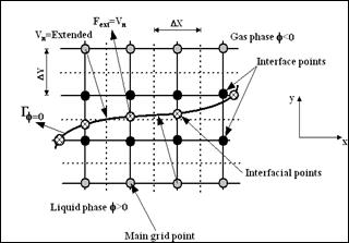
Figure 2. Computational grid and the level set characteristics.
Since the interface is captured implicitly, the level set algorithm is capable of capturing the intrinsic geometrical properties of highly complicated interfaces in a quite natural way. Consequently, the normal vector and the curvature of the interface can be defined as:
![]() (2)
(2)
An important step in the solution algorithm of the level set function is to maintain the level set function as a distance function within the two fluids for all times, especially near the interface region, i.e. the Eikonal equation, ![]() ; should be satisfied in the computational domain. This can be achieved each time step by applying the re-initialization algorithm proposed and described in [4].
; should be satisfied in the computational domain. This can be achieved each time step by applying the re-initialization algorithm proposed and described in [4].
2.1. Fast Marching Method (FMM)
In order to solve the level set equation, Eq. 1, different methods have been also recently developed to overcome the associated numerical problems with the standard level set methods. One of the most important numerical methods is known as the Fast Marching Method (FMM), which has been developed by [18].
The FMM has been mainly developed in order to decrease the computational labour of the standard level set method and maintain the conservative property. The main idea of the FMM is to construct an extension velocity field, Fext, starting from the known normal velocity at the interface Vn, and consequently, the level set equation to be solved is given by:
![]() (3)
(3)
The extension velocity field should satisfy the following equation:
![]() (4)
(4)
2.2. Problem of the Level Set Method
As seen before, one has to solve a simple scalar hyperbolic transport equation in order to obtain the interface properties, such as position, normal vector, and curvature. These parameters play an important role in many physical and engineering phenomena. Therefore, the solution technique of the level set has to be carefully chosen. It can also lead to a stable or unstable solution of the problem under consideration.
As described by [4], when the level set function has been moved with the correct velocity, a steep gradient could be developed. Therefore, the level set must be reinitialized to keep it as a distance function. Without that, the level set function will become irregular and loses its important characteristics.
The resulted numerical diffusion from solution algorithm and reinitialization process of the level set function is directly responsible for the mass conservation error as well as the inaccurate calculation of interface properties. Although, the mass error problem associated with the level set methods could be neglected in many numerical simulations, it will become a very important parameter in others, such as the simulation of two-phase flows. In such cases, this error can affect the physical process, and consequently, it can not be more neglected.
As a general, it is impossible to prevent the level set function from deviating away from a signed distance function. Our goal in this paper is two fold; firstly, the analysis of the reinitialization process, provided by [4], in order to eliminate its disadvantages. Secondly, we turn our attention to the approximation of the space and time derivatives in the level set equation to obtain high accuracy algorithms.
2.3. Reinitialization Process
As mentioned before, the level set function f will move with Eq.(1), using the correct velocity components. The associated problem is that f is no longer a distance function after a period of time, (i.e.,![]() ). In order to keep the level set as a normal distance function for all times, one has to solve the Eikonal equation,
). In order to keep the level set as a normal distance function for all times, one has to solve the Eikonal equation,
![]() (5)
(5)
Many level set methodologies have been developed to solve the above equation, or in otherwise, to keep![]() by the so called reinitialization algorithm. A straightforward way to reinitialize the level set is proposed by [4], that can ensure that f remains a distance function and prevent inaccurate computations near flat/steep regions. This is achieved by performing a pseudo time integration of the following equation:
by the so called reinitialization algorithm. A straightforward way to reinitialize the level set is proposed by [4], that can ensure that f remains a distance function and prevent inaccurate computations near flat/steep regions. This is achieved by performing a pseudo time integration of the following equation:
![]() (6)
(6)
Until a steady state, with the initial conditions
![]() (7)
(7)
![]() is defined as a sign function according to the following equation:
is defined as a sign function according to the following equation:
![]() (8)
(8)
where δ is constant.
The steady state solution is reached when the convergence criterion is achieved, and it is given by:
![]() (9)
(9)
where M ≡ a specified number of grid points and α denotes the prescribed thickness of the interface.
The later reinitialization process works very well and produces the desired signed distance function. However, it is somewhat wasteful of calculation time due to its iterative technique. The steady state solution could not be achieved in some cases, even after a large number of iterations. As a result of these iterations, we refer the most of the associated problems, such as: the movement of the zero level set and consequently the non-conservative mass. By studying the effects of the constants used in the reinitialization process, we have found that, the variable δ, described in Eq.(8), has a large effect on the number of iterations required for the steady state solution and on the mass conservation as well. This constant has no physical meaning, and it is taking as δ = ζΔx, where ζ is a positive number equals one [4]. Our analysis showed that, this constant δ should not be the same from case to case. Through the adjustment of its value to suit the case under consideration, the iteration process takes just one iteration (in the considered cases) until the steady solution is achieved. Fortunately, one need to define the value of δ only at the start of the calculation as this value does not change during the calculation process. For the considered cases, we have found that, good results have been obtained when δ ≤ 17x. This is evident through a reduction of the error in the mass conservation and a saving in the computation time, as the reinitialization process takes only one iteration.
2.4. Numerical Approximation of the Level Set Equation
In the following section, the numerical approximation of the level set method is presented; namely, the temporal derivative and the convective terms. These approximations are relatively new and developed by the present author.
2.4.1. Temporal Derivative
The most common method for level set temporal advection is based on an important family of time-integration techniques which are of a high order of accuracy and provided by Runge-Kutta methods. The Runge-Kutta method was used for the advection scheme presented by [19], and it is used also in the present calculations.
2.4.2. Convection Terms
In the present work, the central difference scheme is applied for the approximation of the convection terms in the level set equation. However, it has been shown that the central difference scheme is failed in two special cases [20], as it produces a miscalculation which propagates outwards as wild oscillations. Therefore, we have to perform these two special cases using our developed algorithm, along with the application of the modified reinitialization process.
3. Numerical Validation
The central difference approximations are applied in the present paper for the convective terms, providing a high order accurate solver compared with the first order upwind scheme used in all the previous level set numerical methods. However, the original work of [20] has showed that the central difference is failed in two specified cases; namely; the movement of a V-front under a dependent gradient normal speed and the movement of a cosine curve under a normal speed along it normal vector field. The central difference approximation produces in such cases a miscalculation at the junction point of the V-front, which propagates outwards as wild oscillation. These oscillations cause blow-up in the code. It should be pointed that these miscalculations have nothing to do with the computational grid distance or the definite time step. Accordingly, it has been concluded that more attention should be given for the gradient term discretization of f in a way that correctly accounts for the entropy condition [20]. Following that, the majority of the papers concerned with the development of the level set technique have applied different orders upwind schemes for solving the level set equation ranging from first-order to second-order ENO or fifth-order WENO scheme. Therefore, we have to perform the specified cases as an important test for our proposed algorithm.
Case I:
The initial configuration of The V-front initial is a "V" formed by rays meeting at (0.5, 0) and can be given by:
 (10)
(10)
The equation of motion for this case is given by:
![]() (11)
(11)
Consider F equals 1 for initial value problem and the difference numerical approximation of the temporal and the spatial derivative is given by:
 (12)
(12)
The expected problem due to central approximation of the gradient term is at x=0.5, where the slope is not defined. In the exact solution, ![]() for all x¹0.5, and this should also hold at x=0.5. However, from Eq.(12) we get the value 1. The Huyghen's construction proposed by [20] sets the correct value for f at x=0.5. Instead of that, we use the reinitialization process to reconstruct the level set according to the other correct values where x¹0.5 after each time step. Consequently, the value at the middle is reconstructed correctly. Figure (3-a) shows the exact solution of the problem. Figure (3-b) shows the calculated results using the central difference without reinitialization and the appearance of the miscalculation at x=0.5 can be seen. The miscalculation of f at x=0.5 is then spread over a wide range in successive time steps. Figure (3-c) shows the calculated results using the central difference approximation with the reinitialization process. It can be observed that as a result of the reinitialization process, the miscalculations disappear. The reconstructive strength of the reinitialization process also holds, when cups with different forms are formed during other front evolution processes, as follows next.
for all x¹0.5, and this should also hold at x=0.5. However, from Eq.(12) we get the value 1. The Huyghen's construction proposed by [20] sets the correct value for f at x=0.5. Instead of that, we use the reinitialization process to reconstruct the level set according to the other correct values where x¹0.5 after each time step. Consequently, the value at the middle is reconstructed correctly. Figure (3-a) shows the exact solution of the problem. Figure (3-b) shows the calculated results using the central difference without reinitialization and the appearance of the miscalculation at x=0.5 can be seen. The miscalculation of f at x=0.5 is then spread over a wide range in successive time steps. Figure (3-c) shows the calculated results using the central difference approximation with the reinitialization process. It can be observed that as a result of the reinitialization process, the miscalculations disappear. The reconstructive strength of the reinitialization process also holds, when cups with different forms are formed during other front evolution processes, as follows next.
(a)
(b)
(c)
Figure 3. The advection of a "V"-front using the central difference approximation for the level set function, (a) the exact solution, (b) without reinitialization, (c) with the reinitialization.
Case II:
Figure 4. The advection of smooth cosine curve along its normal.
The second case that indicates the effectiveness of the proposed level set algorithm is the propagation of an initially simple and smooth cosine curve along its normal vector field with a normal speed Vn=1.0. As seen in [20], the front develops a sharp corner in finite time, and consequently, it is difficult to continue the evolution as the normal vector is ambiguously defined. By using the central difference scheme along with the reinitialization process, the front forms a cusp but the evolution is continued without any disturbances, as seen in Fig. 4.
4. Numerical Results and Discussion
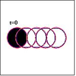
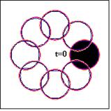
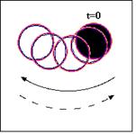
In this section, different simple problems for pure translation and rigid body rotation or oscillation for a circular shape are considered. The oscillation of the circular shape is produced by an oscillatory motion of a simple pendulum whose small amplitude motion is well known. Table 1 gives the summary of the considered test cases and the average area losses of the circular shape over the specified time period. The results of the average area losses of the circular shape, defined over N-iterations as ![]() , reveal that, even for the coarse grid applied, the maximum average area losses is about 4.06e-4, which might be accepted as a numerical error. The preservation of the circular shape during the different movement starting from a specified initial location can be seen in Fig. 5-a, b, c.
, reveal that, even for the coarse grid applied, the maximum average area losses is about 4.06e-4, which might be accepted as a numerical error. The preservation of the circular shape during the different movement starting from a specified initial location can be seen in Fig. 5-a, b, c.
(a)
(b)
(c)
Figure 5. (a) Axial translation of a circular shape, (b) Solid body rotation of a circular shape, (c) Oscillatory pendulum of a circular shape.
Table 1. Summary of the considered data for different movement of a circular shape.
| Movement of Circular Shape | Num. grid | No. of grids equipped by circular shape (D) | Grid dist.Dx, Dy | Initial location of circular shape (xc,yc)|t=0 | Time step Dt | Velocity field; u(x,y), v(x,y) | Average area losses |
| Axial translation | 73×73 | 20 | 0.01 | (17,37) | 35e-4 | (1,0) | 4.907e-5 |
| Rigid body rotation | 73×73 | 20 | 0.01 | (57,37) | 35e-4 | (-1,1) | 4.221e-5 |
| Oscillatory pendulum | 73×73 | 20 | 0.01 | (52,51) | 35e-4 | (cos(Dyc(t)/2.4), sin(Dyc(t)/2.4)) | 4.06e-4 |
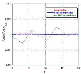
Figure 5. d. Temporal evolution of the normalized area of circular shape under different movements Moreover, the evolution of the normalized area (A(t)/Ainit) of the circular shape as a function of the dimensionless time ![]() is plotted in Fig. 5-d for the different cases considered. The obtained numerical error can be accepted for all movements considered.
is plotted in Fig. 5-d for the different cases considered. The obtained numerical error can be accepted for all movements considered.
5. Droplet Collision inside Microfluidic Device
The dynamics of droplets inside microfluidic devices has been recently extensively investigated; see for more details [21]. The applications are ranged from squeezing, dripping, jetting and flow-focusing devices. The collision dynamics of microfluidic droplets has been recently emerged as an important technology for a wide range of two-phase flow microfluidic applications including encapsulation, chemical synthesis and biochemical assays. More recently, in some micro devices, used in the chemical, pharmaceutical or medical technology or related industries. The results of the collision process are dependent on different factors, such as collision energy, droplet size and the collision angle and distance, see for more details [8,11]. Moreover, the numerical algorithm is described in details in [13].
In the present section, a very complex problem for the droplet collision dynamics in microfluidic device is numerically simulated. The computational domain and the boundary conditions for such problem can be seen in Fig. 6, where two unequally droplets in the so-called head-on collision process.
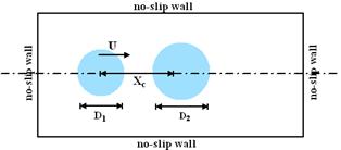
Figure 6. Initial configurations and boundary conditions for two colliding droplets.
The computational domain has 101x101 grid points in x and y directions, respectively. The uniform grid distance is given as Dx=Dy=1.0e-6m. The diameter ratio is considered as D2/D1=2. The time step is chosen as small as possible to ensure the stability of the computational algorithms and equals 0.8e-5s. No-slip boundary conditions are applied for all the boundaries of the computational domain. The adopted numerical algorithm is described in more details in [13].
Initially, two unequally droplets are located head-on in stagnant gas. The moving droplet is called the "ejected" droplet, while the other is called the "target" droplet. The distance between the centres of the droplets is denoted by Xc. The dimensionless numbers control such collision process are the Weber number (We), Reynolds number (Re), and Ohnesorge number (Oh) [22]. All these parameters are dependent on the collision velocity, droplet diameters, and the droplet and the surrounding gas properties.
Simply, two test cases are numerically performed. The dimensionless Weber number for the two cases are as We2/ We1=3, by increasing the colliding velocity while all other properties remain constant. It should be pointed out that the chosen data for our cases is arbitrary.
Figure 7 and Figure 8 show the dynamics of droplet collision process for the considered cases performed with relatively low We reflecting the dynamics of collision process in microfluidic devices. The results show the effects of increasing the colliding velocity of the ejected droplet on the resulting collision process dynamics. Initially, as the ejected droplet approaches the target droplet, it is deformed according to the bag break-up mechanism, while the target droplet is deformed accordingly. As a result of the low colliding velocity, a small amount of air between the two droplets is allowed to form an entrapped air cavity. This cavity can form a bubble inside the target droplet. During the deformation process of the target droplet, the bubble inside goes further in a deformation process due the initial kinetic energy of the ejected droplet and the evolution of the target droplet. Finally, the target droplet is reaches a statistically steady state with an entrapped air bubble involved.
By increasing the colliding velocity, the air bubble is not allowed to form between the two droplets, Fig. 8. Both droplets are nearly deformed according to the bag break-up mechanism. The ejected droplet goes through the cavity formed by the target droplet due its deformation process. The ejected droplet continues its deformation and break-up process until it reaches to equally size droplets with a circular shape. The target droplet is deformed further due to the initial kinetic energy of the ejected droplet and the induced gas flow. However, the target droplet does not break, but it returns to the initial circular shape.
In general, the developed numerical method, applied in the present paper, shows the effectiveness of the level set algorithm in predicting merging and breaking of droplets in natural way without any numerical constraints.
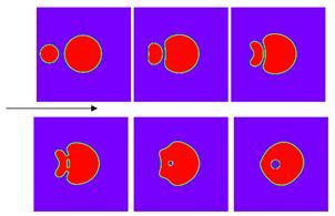
Figure 7. Collision of two unequally droplets at different time steps for We1=0.847.
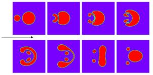
Figure 8. Collision of two unequally droplets at different time steps for We2=3 We1.
6. Conclusions
A high accuracy algorithm for solving the level set equation has been presented. The algorithm is based basically on approximating the convection term with the central difference and using the Rung-Kutta scheme for the time advection. This level set methodology is combined with a reinitialization process in order to keep the level set as a distance function. The accuracy of the algorithm is in the range of the accepted numerical error. This indicates that the present developed numerical method can be applied for predicting the moving fronts in micro- and nano-mechatronic devices.
References
- Nie, Z. H., Seo, M. S., Xu, S. Q., Lewis, P. C., Mok, M., Kumacheva, E., Whitesides, G. M., Garstecki, P. and Stone, H. A., Emulsification in a microfluidic flow-focusing device: effect of the viscosities of the liquids, Microfluid. Nanofluid., 5, 585-594, 2008.
- Yuehao Li, Mranal J. and Krishnaswamy N., Numerical Study of Droplet Formation inside a Microfluidic Flow-Focusing Device, Excerpt from the Proceedings of the COMSOL Conference, Boston, 2012.
- Osher, S.; Sethian, J. A., Fronts propagating with curvature-dependent speed: algorithms based on Hamilton–Jacobi formulations. Journal of Computational, Physics, vol. 79, pp. 12–49, 1988.
- Sussman, M., Smereka, P. and Osher, S., A level set approach for computing solutions to incompressible two-phase flow, J. Comp. Phys. 114, 146–154, 1994.
- Garzon, M, Gray, L.J. and Sethian, J.A., Numerical simulation of non-viscous liquid pinch-off using a coupled level set-boundary integral method, J. of Comp. Physics, 228, 6079–6106, 2009.
- Balabel, A., Binninger, B., Herrmann, M. and Peters, N., Calculation of droplet deformation by surface tension effects using the level set method, Combustion Science and Technology, 174 (11-12), 257–278, 2002.
- Balabel, A., Numerical prediction of droplet dynamics in turbulent flow, using the level set method, International J. of Computational Fluid Dynamics, 25 (5), 239–253, 2011.
- A. Balabel, Numerical simulation of two-dimensional binary droplets collision outcomes using the level set method, International Journal of Computational Fluid Dynamics, vol. 26, no. 1, pp. 1-21, 2012.
- A. Balabel, Numerical modeling of turbulence-induced interfacial instability in two-phase flow with moving interface Applied Mathematical Modelling, vol. 36, pp. 3593–3611, 2012.
- A. Balabel, A Generalized Level Set-Navier Stokes Numerical Method for Predicting Thermo-Fluid Dynamics of Turbulent Free Surface. Computer Modeling in Engineering and Sciences (CMES), vol.83, no.6, pp. 599-638, 2012.
- A. Balabel, Numerical Modelling of Turbulence Effects on Droplet Collision Dynamics using the Level Set Method. Computer Modeling in Engineering and Sciences (CMES), vol. 89, no.4, pp. 283-301, 2012.
- A. Balabel,Numerical modeling of turbulence-induced interfacial instability in two-phase flow with moving interface, Applied Mathematical Modelling, vol. 36, no. 8, pp. 3593-3611, 2012.
- A. Balabel, Numerical prediction of droplet dynamics in turbulent flow, using the level set method. International Journal of Computational Fluid Dynamics, vol. 25, no. 5, pp. 239-253, 2012.
- A. Balabel, Numerical Modelling of Liquid Jet Breakup by Different Liquid Jet/Air Flow Orientations Using the Level Set Method, Computer Modeling in Engineering and Sciences (CMES), vol. 95, no.4, pp. 283-302, 2013.
- Peters, N, Turbulent combustion. Cambridge University Press, Cambridge, UK, 2000.
- Chiu, P. and Lin, Y., A conservative phase field method for solving incompressible two-phase flows, J. of Comp. Physics, vol. 230, pp. 185–204, 2011.
- Hirt, C. W. and Nichols, B. D., Volume of fluid (VOF) method for the dynamics of free boundaries, J. of Computational Physics, vol. 39, pp. 201-225, 1981.
- Adalsteinsson, D. and Sethian, J. A., The Fast Construction of Extension Velocities in Level Set Methods, J. Comp.Phys., vol. 148, pp. 2-22, 1999.
- Shu, C.-W. and Osher, S., Efficient implementation of essentially non-oscillatory shock-capturing schemes II. J. Comp. Phys., vol. 83, pp. 32-78, 1989.
- Sethian J., Level set methods, Cambridge University Press, 1996.
- Taotao Fu., Yining Wu., Youguang Ma, Huai Z.Li, Droplet formation and breakup dynamics in microfluidic flow-focusing devices: From dripping to jetting, Chem. Eng. Sci., vol. 84, pp. 207-217, 2012.
- Bayvel, L. and Orzechowski, Z., Liquid Atomization, Taylor and Francis, London., 1993.


