
International Journal of Economics and Business Administration, Vol. 1, No. 2, September 2015 Publish Date: Aug. 10, 2015 Pages: 120-127
Does Trade Openness Influence Economic Growth?
Fateh Habibi*
Department Economics, Faulty of Humanities and Social Sciences, University of Kurdistan, Sanandaj, Iran
Abstract
The aim of this study is to determine the effects of trade openness on economic growth. We use panel cointegration tests and panel error-correction models (ECM) to explore the causal relationship between trade openness and economic growth for 120 countries over the period 2000-2013. The results of pedroni cointegration test demonstrate that trade openness and economic growth is cointegrated; on the other hand, a long run relationship can be fine among these two variables. We segment the data set into four subpanels according to per capita income classification that distinguishes between low-income, lower-middle-income, upper-middle income and high-income economies. The results suggest that the long-run causality between trade openness and growth runs in four panel groups. The result indicates that bidirectional causalities in the study were observed from real GDP growth to trade openness in all panels except low income groups. Second, unidirectional causation from trade openness to economic growth was obtained in the study for low income economies. The desired growth-led openness and openness-led growth hypothesis can only be supported for Upper middle and high income countries.
Keywords
Trade Openness, Economic Growth, Classification Countries, Panel Data
Received: July 10, 2015
Accepted: August 1, 2015
Published online: August 9, 2015
@ 2015 The Authors. Published by American Institute of Science. This Open Access article is under the CC BY-NC license. http://creativecommons.org/licenses/by-nc/4.0/
1. Introduction
Over the past 60 years, trade liberalization has contributed to increasing the standard of living of billions of people across the world by creating new economic opportunities and lower prices to consumers. An open international trade and investment environment is fundamental to foster economic growth, job creation and prosperity (ICC, 2013). Over the past few years, the world trading system is becoming progressively open and competitive. Tariffs are reducing in both developed and developing countries and restrictions are eliminating. International trade plays an important role in the development of any economy. International trade affects economy through, creates employment, generate capital formation that leads to better living standards in terms of higher level of GDP and GDP per capita (Lewis, 1980). Trade openness can be seen as an important catalyst for the growth and development in an economy. The high degree of trade openness can enhance market access to its goods and services sectors. In addition, there is a positive impact of trade openness on cross border inter and intra-firm trade activities (Turner and Witt, 2001).
The openness improves the efficient allocation of resources through comparative advantage, allows the dissemination of knowledge and technological progress, and encourages competition in domestic and international markets (Chang et al, 2005). The recent empirical growth literature has suggested a wide list of growth determinants, with trade openness among others. Figure 1 show the trade as percentage of GDP. Data from the World Development Indicators, 2015 show that the share of trade in percentage of GDP increased substantially between 2005 (54%) and 2008 (62%), then was driven down by the financial crisis to 52% in 2009, before going up again to 61% in 2013. Figure 1 shows that in 2013, the share of trade in high-income developing economies was higher than the other regions (150%) and another region are developing economies (69%), developed economies (56%), middle income (21%) and low income (8%) respectively.
Figure 2 shows that the growth of GDP countries in Low and middle income courtiers was less affected by the 2008 financial crisis than other regions, such as Developed and high income countries who all experienced negative growth rates in 2009. The low income and middle income countries region recovered from the financial crisis along with the global economy. Economic growth was positive in 2013, back to almost 5% and 6%. Also figure 2 shows that developed economies are the most affected by the crisis with a negative growth rate of 4% in 2009.
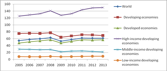
Figure 1. Trade as a percentage of GDP, 2005-2013.
Source: World Bank, World Development Indicators database online, 2015
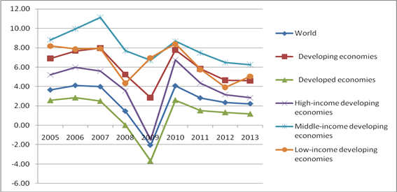
Figure 2. GDP Growth in the world, 2005-2013.
Source: World Bank, World Development Indicators database online, 2015.
2. Literature Review
There are a lot of studies investigating empirical relationship between international trade (trade openness) and economic growth. With regard to a theoretical relationship between openness and growth most of the studies implies the positively effects of trade openness on growth (Romer, 1993; Grossman and Helpman, 1991). Also countries that are more open have a greater ability to catch up to leading technologies of the rest of the world (Barro and Sala-i-Martin, 1995). Some studies concluded that openness played effective role mostly in developed countries whereas many studies concluded that openness can play significant role in less developed countries as well (Dowrick and Golley 2004; Hassan and Kamrul, 2005). Many studies in the literature have proved the importance of international trade for economic growth. Empirical studies prove that international trade is crucial for economic growth of many countries (Kruger, 1980; Marin, 1992; Bahmani-Oskooee and Alse, 1993; Jin, 1995; Xu, 1996; Shan and Sun, 1998; Kulendran and Wilson, 2000; Shan and Willson, 2001; Deme, 2002). Some of these studies, for instance Grossman and Helpman (1991), Lucas (1988), Young (1991) and Rivera–Batiz and Xie (1993), note that trade openness has a negative effect on individual country, while Harrison (1996) documents that trade openness has a strong and positive impact on economic growth.
Although export is a component of GDP and thus leads directly to output growth, many empirical studies have found support for the export-led growth hypothesis (Chow, 1987; Bahmani-Oskooee and Alse, 1993; Xu, 1996) and some others have found a negative relationship (Jung and Marshall, 1985; Darrat, 1986; Ahmed and Kwan, 1991; Dodaro, 1993). Furthermore, some other empirical studies have confirmed the import-led growth hypothesis (Deme, 2002). Exports and imports have also been linked to each other in the empirical literature. Narayan and Narayan (2005) indicate that exports and imports are cointegrated only for 6 out of the 22 least developed countries. Hur and Cheolbeom (2012) has used sample of 90 developed and developing countries for 1958-2003. The results of this study imply that Free trade agreement has insignificant relation with output growth during initial 1-10 years after its launch but finds a significant upward trend among the participating countries.
Jacob Kloster (2015) analyzed trade volume and economic growth in 22 MENA countries using GMM estimator for the period 1960-2011. The results show that trade in services and trade in goods both do increase gross domestic product as trade policy openness and higher ratios of trade volumes to gross domestic product are positively correlated with growth. The interaction between trade in goods and trade in services is negative. This result is surprising given the complementarily between trade in goods and trade in services. Inefficient services, provided mostly by the public sector, and the high cost of key Back bone services such as transport, telecommunications, storage and distribution are important factors that raise the cost of MENA exports, while also impeding trade expansion in the MENA region.
Arif and Ahmad (2012) investigate the relationship between trade openness and economic growth for Pakistan using granger causality for 1972-2010. The results of granger causality test show that there is a bi-directional significant relationship between trade openness and economic growth. Hassan and Kamrul (2005) investigated the casual relationship between trade openness and economic growth and the structure of international trade for Bangladesh. The study explored that there was long-run uni-directional equilibrium relationship between trade openness and economic growth. Yanikkaya (2003) investigated the impact of trade liberalization on per capita income growth for 120 countries using GMM estimator for the time period 1970 to 1997. The results of study showed that openness based on trade volumes were significant and positively related with per capita output growth. However, for developing countries openness based on trade restrictions were significant and positively related with per capita output growth.
Ekanayake, Vogal and Veeramacheneni (2003) checked the causal relationship between output level, inward FDI and exports for a cross-section of both developed and developing countries for period 1960-2001. The study concluded that there was bi-directional causality between export growth and economic growth. Edwards (1998) analyze the relationship between trade policy and total factor productivity (TFP) growth for the period 1980 to 1990 for 93 countries. According to the results of OLS estimates trade openness indexes were significantly and positively associated with TFP growth whereas trade distortion indexes were significantly and negatively associated with TFP growth.
The contributions of this paper are as follows: Firstly, A weak point of literature studies is the absence of a general examination of the causality between openness and economic growth on cross-country level. All these studies investigate the relationship on a certain country level for time series data or sample of a few panel countries. A general panel error correction model has not been applied yet. Therefore, this study aims to address this problem and to re-examine the issue of causal links between trade openness and growth using an error correction model for a panel of 120 countries over the period 2000-2013. This methodological framework allows us to test for bidirectional causality relations from trade openness to GDP and vice versa. We also break down our data set into four subpanels following the World Bank income classification namely; low-income, lower-middle-income, upper-middle income and high-income economies to allow us to investigate income-related affect differences. The empirical results from this study can shed light on the potential impact of trade openness in goods and services, which is seen as a high value-added industry in terms of its diverse linkages with other industries. The remainder of this paper is organized as follows: Section 2 explains methodology. Section 3 presents data and sources. Section 4 presents the empirical results of the panel unit root tests, the panel cointegration tests, and the error-correction model and finally policy implication and conclusion are presented in section 5.
3. Methodology and Data
This section investigates the causal relationship between trade openness and economic growth. The test for relationship and causality between trade openness and economic growth in developing countries will be performed in three steps. First, we use recently developed panel data root test for the order of integration. Second, having established the order of integration in the series, we use heterogeneous panel cointegration test for the long run relationships between the variables. Finally, we apply panel based error correction model to explore the direction of causality between these two variables.
3.1. Panel Unit Root Test
Before panel Granger causality test we uses unit root test to check the stationarity of the time series by using three different statistics proposed by Im, Pesaran and Shin (1997, 2003), Levin, Lin and Chu (2002), Hadri (2000), as the power of individual unit root test can be distorted when the data is short. From among different panel unit root tests developed in the literature, LLC and IPS are the most popular. Both of the tests are based on the ADF principle. However, LLC assumes homogeneity in the dynamics of the autoregressive coefficients for all panel members. In contrast, the IPS is more general in the sense that it allows for heterogeneity in these dynamics.
3.1.1. Levin, Lin and Chu Test (LLC, 2002)
LLC disputed that individual unit root tests have limited power against alternative hypotheses particularly in small samples. LLC suggest a more powerful panel unit root test than performing individual unit root tests for each cross-section. The null hypothesis is that each individual time series contains a unit root against the alternative, that each time series is stationary. In LLC the main hypothesis of panel unit root is as follows:
![]() (1)
(1)
Where ![]() refer to variables lnTO, ln GDP, ∆ refers to first difference, i refers to country and t refers to time period. The hypotheses are as follow:
refer to variables lnTO, ln GDP, ∆ refers to first difference, i refers to country and t refers to time period. The hypotheses are as follow:
![]() (Each individual time series has a unit root)
(Each individual time series has a unit root)
![]() (Each time series is stationary)
(Each time series is stationary)
The LLC test requires a specification of the number of lags used in each cross-section ADF regression (pi). In addition, we must specify the exogenous variables used in the test equations, also select to include no exogenous regressors, or to include individual constant terms (fixed effects), or to employ constants and trends. LLC suggest using their panel unit root test for panels of moderate size with N between 10 and 250 and T between 25 and 250. The proposed LLC test has its limitations. The test crucially depends upon the independence assumption across cross-sections and is not applicable if cross-sectional correlation is present. Second, the assumption that all cross-sections have or do not have a unit root is restrictive.
3.1.2. Im, Pesarn and Shin Test (IPS, 1997, 2003)
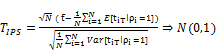
The Levin, Lin and Chu test is restrictive in the sense that it needs ρ to be homogeneous across countries (i). According to Maddala (1999), the null may be fine for testing convergence in growth between countries, but the alternative restricts every country to converge at the same rate. The advantage of IPS test is to permit for a heterogeneous coefficient of lag dependent variable,![]() , and suggest an alternative testing procedure based on averaging individual unit root test statistics (Im et al. 2003). IPS uses an average of the augmented (ADF) tests for each cross-section. The IPS t-bar statistics is defined as the average of the individual ADF statistics as follow:
, and suggest an alternative testing procedure based on averaging individual unit root test statistics (Im et al. 2003). IPS uses an average of the augmented (ADF) tests for each cross-section. The IPS t-bar statistics is defined as the average of the individual ADF statistics as follow:
![]() (2)
(2)
Where, t![]() iis the individual t-statistic for testing
iis the individual t-statistic for testing ![]() for all countries. ). In the general case where the lag order pi may be nonzero for some cross-sections, IPS shows that a properly standardized
for all countries. ). In the general case where the lag order pi may be nonzero for some cross-sections, IPS shows that a properly standardized![]() has an asymptotic N (0, 1) distribution.They then use estimates of its mean and variance to convert t-bar into a standard normal ‘z-bar’ statistic so that conventional critical values can be used to evaluate its significance. The z-bar test statistic for 1-lag is defined as:
has an asymptotic N (0, 1) distribution.They then use estimates of its mean and variance to convert t-bar into a standard normal ‘z-bar’ statistic so that conventional critical values can be used to evaluate its significance. The z-bar test statistic for 1-lag is defined as:
 (3)
(3)
As T![]() followed by N
followed by N ![]() successively, the values of
successively, the values of ![]() and
and ![]() have been computed by IPS through simulations for different values of T and
have been computed by IPS through simulations for different values of T and ![]() i’s. IPS also employs a group mean Lagrange multiplier (LM) test for testing
i’s. IPS also employs a group mean Lagrange multiplier (LM) test for testing ![]() . In Monte Carlo experiments, they show that the average LM and t-statistics have better finite sample properties than the LL test. IPS (2003) provide exact critical values of the t-bar NT statistic for some N,T ranges and for the 1, 5, 10% confidence levels.
. In Monte Carlo experiments, they show that the average LM and t-statistics have better finite sample properties than the LL test. IPS (2003) provide exact critical values of the t-bar NT statistic for some N,T ranges and for the 1, 5, 10% confidence levels.
3.2. Panel Cointegration Test
The concept of cointegration was first introduced into the literature by Granger (1980). Cointegration implies the existence of a long-run relationship between economic variables.
The panel cointegration test, for heterogeneous panels, which are developed by Pedroni (2000) are used in this study due to several advantages: First, it offers efficient estimation of a long run relation among variables, Second, it allows (using the asymptotic properties of non-stationary panels) for considerable heterogeneity among individual section of the panel, Third, the error term can be correlated with the explanatory variables, Fourth, the method is applicable to multiple regressors (Pedroni, 1999). In addition, panel cointegration test permit one to selectively pool the long run in the panel while allowing the short run dynamics between different countries (Pedroni, 2000).
Pedroni (1999) suggested two types of test. The first is based on the within-dimention approach and second is based on the between-dimension approach. The first test includes four statistics namely the panel ![]() -statistic, panel
-statistic, panel ![]() -statistic, panel PP-statistic and the panel ADF-statistic. These statistics pool the autoregressive coefficients across different countries for the unit root tests on the estimated residuals. The second test includes three statistics. They are the group
-statistic, panel PP-statistic and the panel ADF-statistic. These statistics pool the autoregressive coefficients across different countries for the unit root tests on the estimated residuals. The second test includes three statistics. They are the group![]() -statistic, group PP-statistic and group ADF-statistic. These statistics are based on estimators that simply average the individually estimated coefficients of each country.
-statistic, group PP-statistic and group ADF-statistic. These statistics are based on estimators that simply average the individually estimated coefficients of each country.
The seven of Pedroni’s tests are based on the estimated residuals from the following long run model:
![]() (4)
(4)
where![]() are the estimated residuals from the panel regression, i refers to country and t refers to time period.
are the estimated residuals from the panel regression, i refers to country and t refers to time period.
To conduct panel cointagration test requaries two step. First, the cointegration equation is estimated separately for each panel. Second, the residuals are examined with respect to the unit root test. If the null hypothesis is rejected, the long run equilibrium exists. In the group statistics, the autoregressive parameter is permitted to over the cross section. If the null hypothesis is rejected, cointegration holds at least for one individual. The null hypothesis tested is whether ![]() is unity. The seven statistics are normally distributed. The statistics can be compared to appropriate critical values, and if critical values are exceeded then the null hypothesis of no-cointegration is rejected implying that a long run relationship between the variables does exist.
is unity. The seven statistics are normally distributed. The statistics can be compared to appropriate critical values, and if critical values are exceeded then the null hypothesis of no-cointegration is rejected implying that a long run relationship between the variables does exist.
3.3. Panel Causality
Pedroni’s heterogeneous panel cointegration method tests only for the existence of long run relationships. The tests indicate the presence or absence of long run links between the variables, but do not indicate the direction of causality when the variables are cointegrated. If the variables are cointegrated and panel co-integration is found, next step is to apply the Granger causalitytest. For this purpose a panel-based error correction model (ECM) is used to explain the long-run relationship by using the Engle and Granger (1998) procedures with a dynamic error correction: So then, the following models are estimated:
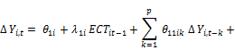
![]() (5)
(5)
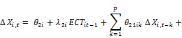
![]() (6)
(6)
where ECT is the error correction term, i refers to country and t refers to time period.
4. Data
Regarding openness there are several variables that can be used to measure the degree of openness. They can be divided into two categories; First, measure of trade share, which is the sum of exports plus imports divided by GDP. The second includes measures of trade barriers that include average tariff rates, export taxes, total taxes on international trade, and indices of non-tariff barriers. To perform a broad panel analysis of a large number of countries and over a long period we select a measure of trade share. We use a balanced panel data set containing 120 countries over the period 2000-2013.
4.1. Trade Openness: TOi,t
Trade measured by the sum of exports and imports as a percentage of GDP at 2005 constant prices. i refers to country and t refers to time period.
4.2. GDP per capita: GDPi,t
GDP per capita is PPP converted GDP per capita at 2005 constant prices in international dollar per person. In addition to the entire panel, we segment the data set into four subpanels according to per capita income. We use the World Bank country classification that distinguishes between low-income economies ($1,045 or less), lower-middle-income economies ($1,046 to $4,125), upper-middle income economies ($4,126 to $12,735), high-income economies ($12,736 or more) (WDI, 2015). Trade openness as a percentage of GDP (Export + Import / GDP) (TO) and GDP per capita growth rate data were taken from the World Bank Development Indicators (World Bank, 2015). Annual time series data covering the period 2000-2013 for which data available was used. i refers to country and t refers to time period.
5. Results and Discussion
In order to determine the presence of a unit root in a panel data setting, we have used the panel unit root test based on the Levin, Lin and Chou (LLC, 2000) and Im, Pesaran and Shin Test (IPS, 1997, 2003) on the panel data. Tables 1 and 2 show the results of the tests at level and first difference for LLC and IPS test respectively. The results indicate that for both variables the level data is non-stationary. The null of unit roots is strongly rejected at the 1% significance level for all series at their first difference. The test statistics of the differenced variables are highly significant and show stationarity. We found that all the test statistics significantly confirm that all series are integrated of order one I(1) according to the LLC and IPS test results.
Table 1. The Results of LLC Panel Unit Root Test.
| Groups | LGDP | LTO | ||||||
| Level | F. Diff | Level | F. Diff | |||||
| C | C+T | C | C+T | C | C+T | C | C+T | |
| Low Income | -1.37 | -1.60 | -4.91* | -6.75* | -2.65 | -2.95 | -5.24* | -5.79* |
| Lower-Middle Income | -1.16 | -2.92 | -5.24* | -4.77* | -3.06 | -1.75 | -7.85* | -9.613* |
| Upper-Middle Income | -2.50 | -1.61 | -6.75* | -6.82* | -1.84 | -1.60 | -4.75* | -6.71* |
| High Income | -2.75 | -1.11 | -8.57* | -5.49* | -2.82 | -2.74 | -5.36* | -4.04* |
Notes: * indicates rejection of the null hypothesis of a unit root at 1% level of significance.
Table 2. The Results of IPS Panel Unit Root Test.
| Groups | LGDP | LTO | ||||||
| Level | F. Diff | Level | F. Diff | |||||
| C | C+T | C | C+T | C | C+T | C | C+T | |
| Low Income | -1.54 | -1.72 | -7.57* | -9.26* | 0.89 | -1.78 | -6.64* | -8.51* |
| Lower-Middle Income | -2.66 | -1.33 | -3.92* | -7.21* | -1.33 | 0.39 | -3.73* | -2.85* |
| Upper-Middle Income | -1.26 | -0.55 | -5.33* | -6.39* | -1.54 | -1.11 | 4.39* | -6.72* |
| High Income | -1.20 | 2.30 | -4.32* | 5.73* | -2.75 | -0.46 | -3.86* | -5.82* |
Notes: * indicates rejection of the null hypothesis of a unit root at 1% level of significance.
Since the panel unit root tests presented above indicate that the variables are integrated of order one I (1), we test for cointegration using the panel cointegration test developed by Pedroni (2004). Table 3 reports the results of Pedroni panel cointegration test. The test contains seven cointegration statistics, the first four based on pooling the residuals along the "within-dimension" which assume a common value for the unit root coefficient, and the subsequent three based on polling the residuals along the "between dimension" which allow for different values of the unit root coefficient. Table 3 presents the results. In all cases the null of no cointegration is rejected at the 1 percent level of significance, On the other hand, there is a long-run relationship between LGDP and LTO for the panel of four gropes namely; low-income economies, lower-middle-income economies, upper-middle income economies and.
Table 4 present the results for the income subpanels, which are low-income economies, lower-middle-income economies, upper-middle-income economies, high-income economies. Generally, all these coefficients are negative and highly significant as expected, so the results show that there exists a long-run relationship and provide evidence of a cointegration relationship between the variables. To investigation granger-causality relationship between Trade openness and economic growth two cases were considered: (i) Trade openness does not Granger-cause GDP growth, and (ii) GDP growth does not Granger-cause trade openness. The empirical results in column with growth (GDP) is dependent variable indicate that trade openness a significant contribution to economic growth in the short run. Specifically, the null hypothesis that tourism does not ‘Granger-cause’ real GDP could be rejected at the 1 percent level in all panel groups. This result is consistent with some previous studies also found that a trade openness-lead growth (Hur and Cheolbeom, 2012; Jacob Kloster, 2015; Hassan and Kamrul, 2005). These results indicate that the trade openness is significant at 1 percent level to Granger-caused economic growth.
Table 3. Pedroni’s Heterogeneous Panel Cointegration Test Results.
| Low Income | Lower-Middle Income | Upper-Middle Income | High Income | |||||
| C | C+T | C | C+T | C | C+T | C | C+T | |
| Panel-v | -5.02* | -3.22* | -3.43* | -5.23* | -4.05* | -6.15* | -6.39* | -4.25* |
| Panel-ρ | -3.56* | -7.85* | -6.19* | -4.23* | -5.91* | -8.24* | -3.49* | -7.08* |
| Panel-t | -4.18* | -6.48* | -4.64* | -5.47* | -4.57* | -6.54* | -5.71* | -6.65* |
| Panel-ADF | -5.24* | -6.74* | -5.15* | -5.66* | -4.74* | -5.25* | -6.96* | -7.24* |
| Group-ρ | -5.11* | -12.41* | -5.64* | -4.09* | -8.31* | -9.73* | -6.65* | -8.62* |
| Group-t | -8.18* | -7.38* | -5.66* | -8.86* | -6.78* | -7.16* | -7.83* | -9.62* |
| Group-ADF | -6.64* | -8.24* | -11.67* | -8.33* | -9.94* | -6.77* | -9.95* | -11.54* |
Notes: All statistics are from Pedroni’s procedure (1999) which is the adjusted values can be compared to the N (0,1) distribution.Panel- v is a nonparametric variance ratio statistic. Panel-ρ and panel-t are nonparametric Phillipes-Perron and t statistics respectively. Panel-adf is a parametric statistics based on the augmented Dickey-Fuller ADF statistic. Group-ρ is analogous to the Phillipes-Perron ρ statistic. Group-t and group-adf are analogous the Phillipes-Perron t statistic and the augmented Dickey-Fuller ADF statistic respectively.
*indicates rejection of the null hypothesis of no-cointegration at 1% level of significance.
After confirming the long run relationship between our variables, next step we use Granger causality analysis taking into account panel error correction model. The results of Panel Granger causality tests are presented in Table 3.
Table 4. Results of Panel Granger Causality test.
| Dependent Variable | ||||
| Groups | Independent Variable | ∆LGDP | ∆LTO | ECMt-i |
| Low Income | ∆LGDP | - | 1. 123(0.1241) | -0.036(0.0372)** |
| ∆LTO | 2.512 (0.0003)* | - | -0.463(0.002)* | |
| Lower-Middle Income | ∆LGDP | - | 2.07(0.4385) | -0.301(0.0021)* |
| ∆LTO | 3.63(0.0042)** | - | -0.054(0.0345)** | |
| Upper-Middle Income | ∆LGDP | - | 4.08(0.0387)** | -0.102(0.0671)** |
| ∆LTO | 3.03(0.0005)* | - | -0.343(0.0001)* | |
| High Income | ∆LGDP | - | 3.37(0.0010)* | -0.453(0.0314)* |
| ∆LTOP | 4.57(0.0021)* | - | -0.234(0.0065)* | |
Notes: * and ** denotes statistical significance at 1% and 5% level respectively.
As expected the error-correction term is negative and significant, indicating that there is a long run relationship between growth and trade openness in 4 panel groups. For example in panel of high income economies, the estimated coefficient of the ECM (-1) is equal to -0.453 and significant at 1 percent level. The rather high coefficient of the ECT suggests that the speed of adjustment back to equilibrium following a disturbance is fairly rapid by 45 percent over the following year. Results of column with (TO) trade openness is dependent variable shows the result of test GDP growth does not Granger-cause tourism. The result indicates that then ull hypothesis that GDP does not ‘Granger-cause’ trade openness fails to reject except in low income economies. Then, the hypothesis of GDP-led Trade openness is valid in Lower-Middle Income, Upper-Middle Income and High Income economies.
This result indicates that a bidirectional causality relationship between trade openness and economic growth in the three groups mention above. Also, bidirectional causalities in the study were observed from real GDP growth to trade openness in all panels except low income groups. Second, unidirectional causation from trade openness to economic growth was obtained in the study for low income economies.
6. Conclusion
This study investigated the possibility of long-run equilibrium relationship and causal relationship between trade openness and economic growth in the income subpanels, which are low-income economies, lower-middle-income economies, upper-middle-income economies, and high-income economies for the period 2000-2013. In a first step we check for stationarity using two common panel unit root tests, the LLC and IPS test. The results of panel unit root test shoe that all variable after first differencing are stationary of order (1). After that we apply a panel cointegration test on openness and growth. As the variables are cointegrated we use panel ECMs to explore the Granger causality between them. The results suggest that the long-run causality between trade openness and growth runs in four panel groups. The short-run adjustment for both directions is negative. The empirical results show that for income-grouped subpanels show that trade openness effect of on economic growth. In summary the overall results of the estimated ECM for the entire panel suggest a bidirectional positive long-run causality between GDP growth and trade openness, indicating that openness promotes economic development and vice versa. The desired growth-led openness and openness-led growth hypothesis can only be supported for Upper middle and high income countries.
References
- A. Lewis. 1980. The slowing down of engine of growth. American Economic review, 70: 555-564.
- Ahmed J, Kwan, AC. 1991. Causality between exports and economic growth. Economics Letters, 37: 246–48.
- Arif, A and Agmad, H. 2012. Impact of Trade openness on output growth: Cointegration and error correction Model approach, International Journal of Economics and Financial Issues, 2(4):479-385.
- Bahmani-Oskooee M, Alse J. 1993. Export growth and economic growth: an application of co-integration and error correction modeling. The Journal of eveloping Areas, 27: 535–42.
- Barro, R.J.; Sala-i-Martin, X. 1995.Economic Growth, McGraw-Hill, Cambridge, MA.
- Bouoiyour, J. 2003. Trade and GDP Growth in Morocco: Short-run or Long-run Causality?, Brazilian Journal of Business and Economics , Vol 3. No. 2, pp. 14-21.
- Chang, R.; Kaltani, L.; Loayza, N. (2009), Openness is Good for Growth: The Role of Policy Complementarities, Journal of Development Economics, Vol. 90, pp. 33-49.
- Chow P C. 1987. Causality between export growth and industrial development: Empirical evidence from the NICs. Journal of Development Economics, 36: 55–63.
- Darrat AF. 1986. Trade and development: the Asian experience. Cato Journal 6: 695–99.
- Deme M. 2002. An examination of the trade-led growth hypothesis in Nigeria: a Co-integration, causality, and impulse response analysis. The Journal of Developing Areas, 36: 1–15.
- Dowrick, S. and Golley, J. 2004. Trade openness and growth: Who benefits? Oxford Review of Economic Policy, 20(1): 38-56.
- Dodaro S. 1993. Exports and growth: a reconsidera-tion of causality. The Journal of Developing Areas, 27: 227–44.
- Dollar, D.; Kraay, A. 2002. Growth is good for the poor. Journal of Economic Growth, 7(3): 195-- 225.
- Ekanayake, Vogal and Veeramacheneni. 2003. Openness and economic growth: empirical evidence on the relationship between output, inward FDI, and trade. Journal of Business Strategies, 20.
- Jin CJ. 1995. Export-led growth and the four little dragons. The Journal of International Trade and Economic Development, 4: 203–15.
- Jung WS, Marshall PJ. 1985. Exports, growth and causality in developing countries. Journal of Development Economics, 18: 1–12.
- Harrison. 1996. Openness and growth: A time series cross country analysis for developing countries. National Bureau of Economic Research. Working paper no.5221.
- Hassan and Kamrul, A F. 2005. Trade openness and economic growth: Search for a Causal Relationship. South Asian Journal of Management. Retrieved on 25th December,2010 from http://findarticles.com/p/articles/mi_qa5483/is_200510/ai_n21363857/?tag=content;col1.
- Hsiao, M.W. 1987. Tests of causality and exogeneity between export growth and economic growth, Journal of Economic Development, 12: 143--159.
- Im, K.S.; Pesaran, M.H.; Shin, Y. 2003. Testing for unit roots in heterogeneous panels, Journal of Econometrics, 115(1): 53-74.
- Grossman, G.M.; Helpman, E. 1991. Innovation and Growth in the Global Economy, Cambridge, MA: MIT Press.
- Krueger AO. 1980. Trade policy as an input to development. American Economic Review, 70: 288–292.
- Levin, A.; Lin, C.F.; Chu, C.S.J. 2002. Unit root tests in panel data: asymptotic and finitesample properties, Journal of Econometrics, 108(1): 1-24.
- Marin D. 1992. Is the export-led hypothesis valid for industrialized countries? Review of Economics and Statistics, 74: 678–688.
- Narayan PK, Narayan S. 2005. Are exports and imports co-integrated? Evidence from 22 least developed countries. Applied Economics Letters, 12: 375–78.
- Narayan PK, Smyth R. 2004. The relationship between the real exchange rate and balance of payments: empirical evidence for China from co-integration and causality testing. Applied Economic Letters, 11: 287–91.
- Pedroni, P. 1999. Critical Values for Cointegration Tests in Heterogeneous Panels with Multiple Regressors, Oxford Bulletin of Economics and Statistics, 61: 653-70.
- Pedroni, P. 2004. Panel Cointegration: Asymptotic And Finite Sample Properties Of Pooled Time Series Tests With An Application To The PPP Hypothesis, Econometric Theory, Cambridge University Press, 20(3): 97-625.
- Romer. 1993. Two strategies for economic development: Using ideas and producing ideas, proceedings of the World Bank annual conference on development economics, 1992, ed.Summers, L.H; Shah, S., pp. 63--91. Washington, D.C.: World Bank.
- Sala-i-Martin, X. 1997. I Just Ran Two Million Regressions, The American Economic Review, 87(2): 178-183.
- Shan JZ, Sun F. 1998. Export-led growth hypothesis for Australia: an empirical re-investigation. Applied Economics Letters, 5: 423–8.
- World Bank. 2015. http://data.worldbank.org/about/country-and-lending-groups%23Low_income.
- Xu X. 1996. On the causality between export growth and GDP growth: an empirical re-investigation. Review of International Economics, 4: 172-184.


