
International Journal of Economics and Business Administration, Vol. 1, No. 2, September 2015 Publish Date: Jun. 17, 2015 Pages: 48-54
A Portfolio of Two Securities
P. N. Brusov1, *, T. V. Filatova2, N. P. Orekhova3
1Applied Mathematics Department, Financial University under the Government of Russian Federation, Moscow, Russia
2Public Administration and Municipal Management, Financial University under the Government of Russian Federation, Moscow, Russia
3High school of Business, Southern Federal University; Investment and Taxation Laboratory, Research Consortium of Universities of the South of Russia, Rostov-on-Don, Russia
Abstract
The main objective of any investor is to ensure the maximum return on investment. During the realization of this goal at least two major problems appear: the first, in which of the available assets and in what proportions investor should invest. The second problem is related to the fact that, in practice, as is well known, a higher level profitability is associated with a higher risk. Therefore, an investor can select an asset with a high yield and high risk or a more or less guaranteed low yield. Two these selection problems constitute a problem of investment portfolio formation, which decision is given by portfolio theory. In this paper the detailed theory of portfolio of the two securities, which represents a simple case, containing, however, all the main features of more common Markowitz and Tobin portfolios has been developed by us. It appears that when selecting anti-correlated or non-correlated securities, you can create a portfolio with the risk, lower, than risk of any of the securities of portfolio, or even zero-risk portfolio (for anti-correlated securities).
Keywords
A Portfolio of Two Securities, Correlated, Anti-Correlated, Non-Correlated Securities
Received:May 6, 2015
Accepted: May 16, 2015
Published online: June 18, 2015
@ 2015 The Authors. Published by American Institute of Science. This Open Access article is under the CC BY-NC license. http://creativecommons.org/licenses/by-nc/4.0/
Contents
1. A Portfolio of Two Securities 1.1. A Case of Complete Correlation 1.2. Case of Complete Anticorrelation 1.3. Independent Securities 1.4. Three Independent Securities 2. Risk–Free Security 3. Portfolio of a Given Yield (or Given Risk) 3.1. Case of Complete Correlation ( ) and Complete Anticorrelation (
 ) 3.2. Case of Complete Correlation () 3.3. Case of Complete Anticorrelation () 3.4. Case of Independent Securities (
 ) 4. Conclusion
1. A Portfolio of Two Securities
1.1. A Case of Complete Correlation
In a case of complete correlation
![]() . (1)
. (1)
For the square of the portfolio risk (dispersion), we have
![]() =
=
![]() =
=![]() . (2)
. (2)
Extracting the square root from both sides, we obtain for portfolio risk
![]() . (3)
. (3)
Since all variables are nonnegative, the sign of the module can be omitted
![]() . (4)
. (4)
Substituting ![]() , accounting
, accounting ![]() , we get
, we get
![]() . (5)
. (5)
This is the equation of the segment (АВ), where points A and B have the following coordinates: ![]()
![]() . t runs from 0 to 1. At
. t runs from 0 to 1. At ![]() portfolio is at point A, and at
portfolio is at point A, and at ![]() – at the point B. Thus, the admissible set of portfolios in the case of complete correlation of the securities is a segment (AB) (Fig. 1).
– at the point B. Thus, the admissible set of portfolios in the case of complete correlation of the securities is a segment (AB) (Fig. 1).
If an investor forms a portfolio of minimal risk, he must incorporate in it one type of paper that has less risk, in this case, the paper A, and the portfolio in this case is ![]() . Portfolio yield (effectiveness)
. Portfolio yield (effectiveness) ![]() .
.
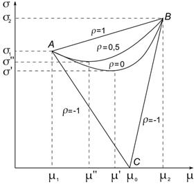
Fig. 1. The dependence of the risk of the portfolio of two securities on its effectiveness for fixed parameters of both securities and with increase in the correlation coefficient from –1 to 1.
With a portfolio of maximum yield, it is necessary to include in it only securities with higher income, in this case, the paper B, and the portfolio in this case is ![]() . Portfolio yield
. Portfolio yield ![]() .
.
1.2. Case of Complete Anticorrelation
In the case of complete anticorrelation
![]() . (6)
. (6)
For the square of the portfolio risk (dispersion), we have
![]() =
=
 =
= . (7)
. (7)
Extracting the square root of both sides, we obtain for portfolio risk
![]() . (8)
. (8)
Admissible set of portfolios in the case of complete anticorrelation of securities consists of two segments (А,С) and (В,С) (Fig. 1). In this case a risk–free portfolio (point C) can exists.
Let us find a risk–free portfolio and its profitability.
From (8) one has
![]() . (9)
. (9)
Substituting in (9) ![]() , we get
, we get
![]() ,
,
![]() . (10)
. (10)
And
![]() . (11)
. (11)
Thus, free–risk portfolio has the form
![]() , (12)
, (12)
and its yield is equal to
![]() . (13)
. (13)
Note that the risk–free portfolio does not depend on the yield of securities and is determined solely by their risks, and the pricing share of one security is proportional to the risk of another.
Since ![]() , then, all admissible portfolios are located inside
, then, all admissible portfolios are located inside
(![]() ), or on the boundary (
), or on the boundary (![]() ), of the triangle ABC.
), of the triangle ABC.
Example 1
For a portfolio of two securities with yield and risk, respectively, ![]() and
and ![]() in the case of complete anticorrelation found risk–free portfolio and its profitability.
in the case of complete anticorrelation found risk–free portfolio and its profitability.
First, using the formula (4.30), we find a risk–free portfolio
![]() .
.
Then by the formula (4.31) we find its yield ![]() .
.
It is seen that the portfolio yield has an intermediate value between the yields of both securities (but portfolio is risk–free!). One can check the results for portfolio yield, calculating it by the formula (4.8) ![]() .
.
1.3. Independent Securities
For independent securities
![]() . (14)
. (14)
For the square of the portfolio risk (variance), we have
![]() . (15)
. (15)
Let us find a minimum–risk portfolio and its profitability and risk. For this it is necessary to minimize the objective function
![]() (16)
(16)
under condition
![]() . (17)
. (17)
This is the task of a conditional extremum which is solved using the Lagrange function
![]() . (18)
. (18)
To find the stationary points we have the system
 , (19)
Subtracting the first equation from the second, we obtain
![]() . (20)
. (20)
Next, using the third equation, we have
![]() . (21)
. (21)
Hence
![]() ,
, ![]() . (22)
. (22)
Portfolio
![]() , (23)
, (23)
and its yield
![]() . (24)
. (24)
The portfolio risk is equal to
 (25)
(25)
Note that in the case of three securities there is no the direct analogy with (23) (see 1.4).
Example 2
Using formula (25) it is easy to demonstrate the effect of diversification on portfolio risk. Suppose a portfolio consists of two independent securities with risks ![]() and
and ![]() , respectively. Let us calculate the portfolio risk by using formula (25)
, respectively. Let us calculate the portfolio risk by using formula (25)
![]() (26)
(26)
Thus, the portfolio risk
![]() (27)
(27)
turns out to be lower than the risk of each of the securities (0.1; 0.2). This is an illustration of the principle of diversification: with "smearing" of the portfolio on an independent securities, risk is reduced.
1.4. Three Independent Securities
Although this case goes beyond the issue of a portfolio of two securities, we consider it here as a generalization of the case of a portfolio of two securities.
For independent securities
![]() . (28)
. (28)
![]() . (29)
. (29)
We find a minimum–risk portfolio, its profitability and risk. For this it is necessary to minimize the objective function
![]() (30)
(30)
under condition
![]() . (31)
. (31)
This is a task on conditional extremum, which is solved using the Lagrange function.
Let us write the Lagrange function and find its extremum
![]() . (32)
. (32)
To find the stationary points we have the system
 (33)
(33)
Subtracting from the first equation the second one, then the third one, we obtain
![]() ,
,
![]() .
.
Hence
![]() . (34)
. (34)
Substituting (34) into the normalization condition
![]() , (35)
, (35)
we get
![]() . (36)
. (36)
Hence
 . (37)
Substituting this ![]() value in (34), we get the rest two components of the portfolio
value in (34), we get the rest two components of the portfolio
![]() , (38)
, (38)
![]() . (39)
. (39)
The portfolio has the form
![]() , (40)
, (40)
and its yield is equal to
![]() . (41)
. (41)
Portfolio risk is equal to
 (42)
(42)
Example 3
For a portfolio of three independent securities with yield and risk ![]() ,
, ![]() and
and ![]() respectively, find the minimum risk portfolio, its risk and yield. Portfolio of minimum risk is given by (40)
respectively, find the minimum risk portfolio, its risk and yield. Portfolio of minimum risk is given by (40)
![]()

So, ![]()
Risk of portfolio of minimum risk is found by formula (42)

Finally, yield of portfolio of minimum risk is found by formula (41)
![]()

It is seen that the portfolio risk is less than the risk of each individual security and a portfolio yield is more than the first security yield, a little less than the yield of the second security and less than the yield of third security.
2. Risk–Free Security
Let one of the two portfolio securities to be risk–free. Portfolio of n–securities, including risk–free one, is named after Tobin, who has investigated this case for the first time. Considering portfolio has properties which are substantially different from those of the portfolio, consisting only of risky securities. Here we consider the effect of the inclusion of a risk–free securities into the portfolio of two securities.
Thus, we have two securities: 1![]() and 2
and 2![]() , with
, with ![]() (otherwise it would be necessary to form a portfolio
(otherwise it would be necessary to form a portfolio ![]() consisting only of the risk–free securities, and we would have a risk–free portfolio of maximum yield).
consisting only of the risk–free securities, and we would have a risk–free portfolio of maximum yield).
We have the following equations:
 (43)
(43)
From these equations it is easy to get an admissible set of portfolios
![]()
which is a segment
![]()
![]() . (44)
. (44)
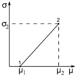
Fig. 2. Admissible set of portfolios, consisting of two securities, one of which is risk–free.
At ![]() portfolio is at a point 1
portfolio is at a point 1![]() , and at
, and at ![]() at a point 2
at a point 2![]() (Fig. 2).
(Fig. 2).
Although this case is very simple, it is nevertheless possible to draw two conclusions:
1) the admissible set of portfolios does not depend on the correlation coefficient (although usually risk–free securities considered to be uncorrelated with the other (risky) securities.
2) the admissible set of portfolios has been narrowed from a triangle to the interval.
Note that a similar effect occurs in the case of Tobin’s portfolio.
In conclusion, we present the dependence of yield and risk of the portfolio on the share of the risk–free securities (Fig. 3).
It is evident that the portfolio risk decreases linearly with ![]() : from
: from ![]() at
at ![]() to zero at
to zero at ![]() , at the same time yield also decreases linearly with
, at the same time yield also decreases linearly with ![]() : from
: from ![]() at
at ![]() to
to ![]() at
at ![]() .
.
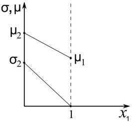
Fig. 3. Dependence of yield and risk of the portfolio on the share of the risk–free security ![]() .
.
3. Portfolio of a Given Yield (or Given Risk)
In the case of a portfolio of two securities, given yield or its risk identifies portfolio uniquely (except the case ![]() , when only the given portfolio risk uniquely identifies portfolio itself, see below for details).
, when only the given portfolio risk uniquely identifies portfolio itself, see below for details).
Under the given yield (effectiveness) of the portfolio, it is uniquely defining as the solution of the system
 (45)
(45)
and under the given portfolio risk, it is uniquely defining as the solution of the system
 (46)
(46)
Therefore, in the case of a portfolio of two securities it is not necessary to talk about the minimal boundary (minimal risk portfolio for its given effectiveness).
Let us consider the first case – the given yield of the portfolio.
We will assume that ![]() . The portfolio is uniquely defined as the solution of the system (45)
. The portfolio is uniquely defined as the solution of the system (45)
Expressing ![]() from the second equation and substituting it in the first equation, we get
from the second equation and substituting it in the first equation, we get
![]() .
.
Hence, we find
![]() , . (47)
, . (47)
Substituting these expressions into the expression for the squared portfolio risk we obtain
 . (48)
Sometimes this equation mistakenly is called by the equation of the minimum boundary. In fact, this equation describes the connection of portfolio risk to its effectiveness.
Only at ![]() , when the equality
, when the equality ![]() is valid for all the values of
is valid for all the values of ![]() and
and ![]() and the feasible set of portfolios is narrowing from the triangle to (vertical) segment, we can speak of the minimal boundary, which in this case consists of a single point
and the feasible set of portfolios is narrowing from the triangle to (vertical) segment, we can speak of the minimal boundary, which in this case consists of a single point ![]() (at
(at ![]() ) or
) or ![]() (at
(at ![]() ).
).
Let us consider different limiting cases, considered by us above.
3.1. Case of Complete Correlation (![]() ) and Complete Anticorrelation (
) and Complete Anticorrelation (![]() )
)
As it is known, the correlation coefficient, does not exceed unity on absolute value, so let us study equation (48) for the extreme values ![]() .
.
First, we present general considerations.
For![]() it is known, that random variables
it is known, that random variables ![]() and
and ![]() are linearly dependent. Without loss of generality we can assume that
are linearly dependent. Without loss of generality we can assume that ![]() . Then, a portfolio yield can be written as follows
. Then, a portfolio yield can be written as follows
![]() . (49)
. (49)
Therefore,
![]() ,
, ![]() . (50)
. (50)
After elimination of the parameter ![]() we obtain the following relation
we obtain the following relation
![]() , (51)
, (51)
i.e. risk, as a function of yield will take the form of a segment or angle (Fig. 1). Now let’s examine the equation (48) in cases ![]() .
.
3.2. Case of Complete Correlation (![]() )
)
![]() (52)
(52)
3.3. Case of Complete Anticorrelation (![]() )
)
![]() (53)
(53)
3.4. Case of Independent Securities (![]() )
)
Equation (48) takes the form
![]() . (54)
. (54)
It could be shown that for intermediate values of the correlation coefficient ![]() portfolio risk as a function of its efficiency has the form
portfolio risk as a function of its efficiency has the form
![]() . (55)
. (55)
If one finds the shape of the dependence of risk portfolio on its effectiveness for a given portfolio ![]() , but for different values of the correlation coefficient,
, but for different values of the correlation coefficient, ![]() , then we can come to the following conclusion:
, then we can come to the following conclusion: ![]() decrease when the correlation coefficient increase from –1 to 1 .
decrease when the correlation coefficient increase from –1 to 1 .
In this case, a plot of the risk portfolio of its effectiveness is becoming more elongated along the horizontal axis, i.e. for a fixed change in the expected yield ![]() , increase in the risk
, increase in the risk ![]() becomes smaller (Fig. 1).
becomes smaller (Fig. 1).
If we also assume that ![]() , and therefore
, and therefore ![]() , it is implied from the first formula (45) that
, it is implied from the first formula (45) that ![]() under the assumption
under the assumption ![]() , as
, as ![]() is their convex combination. Portfolios are part of the boundary of AMB, namely, the part that connects the points
is their convex combination. Portfolios are part of the boundary of AMB, namely, the part that connects the points ![]() and
and ![]() (Fig. 1).
(Fig. 1).
Thus, in the case ![]() and under the additional assumption that
and under the additional assumption that ![]() the set of portfolios is a hyperbola, or pieces of broken lines connecting the points
the set of portfolios is a hyperbola, or pieces of broken lines connecting the points ![]() and
and ![]() .
.
4. Conclusion
The detailed theory of portfolio of the two securities, which represents a simple case, containing, however, all the main features of more common Markowitz and Tobin portfolios has been developed by us. It appears that when selecting anti-correlated or non-correlated securities, one can create a portfolio with the risk, which is lower, than risk of any of the securities of portfolio, or even zero-risk portfolio (for anti-correlated securities).
References
- Brusov, P. N., Filatova, T. B., Orekhova, N. P. & Eskindarov (2015). Modern corporate finance, investments and taxation (378 pp.), Springer International Publishing, Switzerland.
- Brusov P, Brusov PP, Orehova N, Skorodulina S (2010) Financial mathematics for bachelor . KNORUS, Moscow, 224
- Brusov P, Brusov PP, Orehova N, Skorodulina S (2012) Tasks on Financial mathematics for bachelor . KNORUS, Mow, 285
- Brusov P Filatova T (2014) Financial mathematics for masters. KNORUS, Moscow, 480
- Markowitz, H.M. (March 1952). "Portfolio Selection". The Journal of Finance 7 (1): 77–91.doi:10.2307/2975974.JSTOR2975974.
- Markowitz, H.M. (1959).Portfolio Selection: Efficient Diversification of Investments. New York: John Wiley & Sons. (reprinted by Yale University Press, 1970,ISBN 978-0-300-01372-6; 2nd ed. Basil Blackwell, 1991,ISBN 978-1-55786-108-5)
- Tobin, James (1958). Liquidity preference as behavior towards risk, The Review of Economic Studies, 25, 65-86.
- .Tobin, James (1992) The New Palgrave Dictionary of Finance and Money, v. 2, pp.770–79 & inThe New Palgrave Dictionary of Economics. 2008, 2nd Edition
- Brusov, P., Filatova, T., Orehova, N., & Brusova, N. (2011).Weighted average cost of capital in the theory of Modigliani–Miller, modified for a finite life-time company.Applied Financial Economics, 21, 815–824.http://dx.doi.org/10.1080/09603107.2010.537635
- Brusov, P., Filatova, T., Orehova, N., Brusov, P. P., & Brusova, N. (2011a). Influence of debt financing on the effectiveness of the investment project within Modigliani–Miller theory. Research Journal of Economics, Business and ICT, 2, 11–15
| 1. | ||
| 1.1. | ||
| 1.2. | ||
| 1.3. | ||
| 1.4. | ||
| 2. | ||
| 3. | ||
| 3.1. | ||
| 3.2. | ||
| 3.3. | ||
| 3.4. | ||
| 4. | ||


