
International Journal of Economics and Business Administration, Vol. 1, No. 2, September 2015 Publish Date: Jul. 3, 2015 Pages: 59-70
Optimizing of the Investment Structure of the Telecommunication Sector Company
P. N. Brusov1, *, T. V. Filatova2, N. P. Orekhova3, A. P. Brusova4, V. L. Kulik4
1Applied Mathematics Department, Financial University under the Government of Russian Federation, Moscow, Russia
2Dean of GMM Faculty, Financial University under the Government of Russian Federation, Moscow, Russia
3High School of Business, Southern Federal University, Investment and Taxation Laboratory, Research Consortium of Universities of the South of Russia,Rostov-on-Don, Russia
4Management Department, Financial University under the Government of Russian Federation, Moscow, Russia
Abstract
In this paper developed by the authors models of evaluation of the dependence of effectiveness of investments on debt financing are applied for the analysis of investments of one of the biggest telecommunication company of Russia for 2010-2012 years from the point of view of optimal structure of investment. The analysis revealed, that only in 2011 the company's investment structure was close to the optimal.
Keywords
Investment Projects with Arbitrary Duration, Effectiveness of Investment Project, Optimal Leverage Level, Taxes Impact
Received:May 3, 2015
Accepted: May 28, 2015
Published online: June 30, 2015
@ 2015 The Authors. Published by American Institute of Science. This Open Access article is under the CC BY-NC license. http://creativecommons.org/licenses/by-nc/4.0/
Contents
1. Introduction 2. Investment Analysis and Recommendations for Telecommunication Company "Nastcom Plus" 2.1. The Dependence of NPV on Investment Capital Structure 2.2. The Dependence of NPV on the Equity Capital Value and Coefficient b 2.3. Conclusions 3. Effects of Taxation on the Optimal Capital Structure of Companies in the Telecommunication Sector 4. Conclusions
1. Introduction
Investments in tangible and intangible assets play an important role in the activities of any company. They are a necessary condition for structural adjustment and economic growth, provide the creation of new and enhancement of existing basic funds and industries. The role of investment, which is always the one of the most important, is increased many times at the current stage.
For example, in Russia a priority of budget will be the reduced of dependence of the price of oil and gas. The main issue, that help at least to start the movement on this way are, of course, investments. In this way, the role of investment at the present stage is indeed increasing dramatically. In this regard, the role of evaluation of efficiency of investment projects, which in the context of scarcity and limited investment resources allow choose for the realization of the most effective projects, increases. Since virtually all investment projects use debt financing, the purpose of the study of impact of debt financing, capital structure on the efficiency of investment projects, determining of the optimal level leverage - always actual, and, of course, is especially actual at the present time.
Hope to determine the optimal capital structure, in which one or more parameters of efficiency of the project (NPV, IRR, etc.) are maximum, more than half a century has encouraged researchers to deal with the issue. Some of the major problems in the assessment of the effectiveness of the projects are the following :
● What financial flows and how it is necessary to take into account when calculating parameters of efficiency of the project (NPV, IRR, etc. );
● how many discount rate should be used for discounting of financial flows associated with investments;
● how correctly to determine these discount rate.
Discussion concerning the first two problems is still continuing. On the third issue, one needs to note that, in recent years there has been a significant progress in the more correct determining of the cost of the equity capital of the company and its weighted average cost, which as time and are the discount rate when evaluating the NPV of the project. The progress is associated with work performed by Brusov, Filatova and Orekhova (Brusov P, Filatova T, Orehova N, Eskindarov M 2015; Brusov et al 2011a,b,c,d,e; 2012 a,b; 2013 a,b,c; 2014 a,b; Filatova et al 2008), in which the general theory of capital cost of the company (equity cost as well as weighted average cost) was established and its dependence on leverage and on life-time of company was found for the companies with arbitrary life-time. The main difference between their theory and theory by Modigliani and Miller is that former one waives from the perpetuity of the companies, that leads to significant differences of a new theory from theory of Nobel laureates Modigliani and Miller (Modigliani et al 1958, 1963, 1966).
The lack of modern methods of evaluation of effectiveness of investment projects with account of the debt financing, with the correct assessment of discount rate, used in investment models, has identified the need for research. The establishment of such modern models, considering problem from the point of view of equity capital owners as well as from the point of view of equity and debt capital owners, with the use of modern theory by Brusov, Filatova and Orekhova of assess of the equity capital cost and weighted average cost of capital of the company (Modigliani et al 1958, 1963, 1966), which play the role of discount rate in the investment models, can significantly contribute to the problem of the assessment of investment projects effectiveness.
2. Investment Analysis and Recommendations for Telecommunication Company "Nastcom Plus"
Based on the method, developed by the authors (Brusov P, Filatova T, Orehova N, Eskindarov M 2015; Brusov et al 2011a,b,c,d,e; 2012 a, b; 2013 a,b,c; 2014 a, b; Filatova et al 2008) let us analyze the efficiency of investments of one of the leading companies in the telecommunication sector "Nastcom Plus" for 2010-2012 years from the point of view of optimal structure of investment. The source data for the analysis are presented in Table. 1
Table 1. Data of the company "Nastcom Plus" for 2010-2012 years.
| Indicator | 2010 | 2011 | 2012 |
| Investment I, million dollars | 1.124 | 2.05 | 2.763 |
| Revenue, million dollars | 7 204. 335 | 8 232.172 | 9 418.773 |
| Net operating income for the year before taxing, NOI, million dollars | 2 161.3 | 2 469.174 | 2 826 |
| Equity cost at zero leverage, k0, % | 23.67 | 23.67 | 23.67 |
| Debt cost | 8.26 | 7.4 | 6.69 |
| Return-on-investment for one year, β = I / NOI | 1.92 | 1.204 | 1.02 |
| Amount of debt financing , % | 35 | 50 | 50 |
| Amount of equity, % | 65 | 50 | 50 |
| Leverage level, L | 0.54 | 1 | 1 |
| Amount of equity capital S, million dollars | 730.6 | 1 025 | 1 381.5 |
Quantity k0 is the equity cost of financially independent company (or equity cost at zero leverage) and for "Nastcom Plus" is equal to 23,67% (Brusova 2011). Here are also calculated dependence of weighted average cost of capital WACC and the equity cost ![]() on leverage (Fig. 1 ).
on leverage (Fig. 1 ).
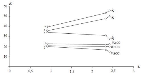
Fig. 1. Dependence of weighted average cost of capital WACC and the equity cost ![]() on leverage: 1, 4 – within Brusov–Filatova–Orekhova theory; 2, 5 – within Modigliani – Miller theory; 3, 6 – within traditional approach.
on leverage: 1, 4 – within Brusov–Filatova–Orekhova theory; 2, 5 – within Modigliani – Miller theory; 3, 6 – within traditional approach.
2.1. The Dependence of NPV on Investment Capital Structure
Analysis of investment will be continued with use of the formula provided in the works (Brusov P, Filatova T, Orehova N, Eskindarov M 2015; Brusov et al 2011a,b,c,d,e; 2012 a,b; 2013 a,b,c; 2014 a,b; Filatova et al 2008):
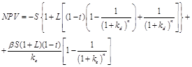 , (1)
, (1)
where
NPV – net present value;
S – equity capital amount;
L – leverage level;
t – tax on profit rate;
kd – debt cost;
n – project duration;
β – return-on-investment for one year;
ke – equity cost.
Analysis of investments in 2010 year Using company's data (Table 1 ), we compute the WACC, ke and NVP (Tables 2–4, Figs. 1 and 2).
Table 2. Weighted average cost of capital, WACC, in 2010 year.
| Project Duration n | Leverage level L | ||||||||||
| 0 | 0.5 | 1 | 1.5 | 2 | 2.5 | 3 | 3.5 | 4 | 4.5 | 5 | |
| 2 | 0.2367 | 0.2284 | 0.2242 | 0.2217 | 0.2201 | 0.2189 | 0.2180 | 0.2173 | 0.2167 | 0.2163 | 0.2159 |
| 5 | 0.2367 | 0.2262 | 0.2209 | 0.2177 | 0.2156 | 0.2141 | 0.2130 | 0.2121 | 0.2114 | 0.2108 | 0.2103 |
| 7 | 0.2367 | 0.2256 | 0.2199 | 0.2166 | 0.2143 | 0.2127 | 0.2116 | 0.2106 | 0.2099 | 0.2093 | 0.2087 |
| 10 | 0.2366 | 0.2250 | 0.2190 | 0.2155 | 0.2131 | 0.2114 | 0.2101 | 0.2091 | 0.2083 | 0.2076 | 0.2071 |
Table 3. Equity cost ke in 2010 year.
| project duration n | Leverage level L | ||||||||||
| 0 | 0.5 | 1 | 1.5 | 2 | 2.5 | 3 | 3.5 | 4 | 4.5 | 5 | |
| 2 | 0.2367 | 0.3096 | 0.3824 | 0.4552 | 0.5280 | 0.6008 | 0.6736 | 0.7464 | 0.8192 | 0.8920 | 0.9649 |
| 5 | 0.2367 | 0.3063 | 0.3758 | 0.4452 | 0.5147 | 0.5841 | 0.6536 | 0.7230 | 0.7925 | 0.8619 | 0.9314 |
| 7 | 0.2367 | 0.3053 | 0.3738 | 0.4423 | 0.5107 | 0.5791 | 0.6480 | 0.7165 | 0.7850 | 0.8535 | 0.9220 |
| 10 | 0.2366 | 0.3044 | 0.3720 | 0.4396 | 0.5071 | 0.5746 | 0.6422 | 0.7097 | 0.7772 | 0.8447 | 0.9122 |
Table 4. Net present value NPV in 2010 year , million dollars.
| Project duration n | Leverage level L | ||||||||||
| 0 | 0.5 | 1 | 1.5 | 2 | 2.5 | 3 | 3.5 | 4 | 4.5 | 5 | |
| 2 | 910.5 | 1 181.8 | 1 358.3 | 1 458.5 | 1 496.3 | 1 482.8 | 1 426.6 | 1 334.6 | 1 212.4 | 1 064.5 | 894.5 |
| 5 | 2 371.6 | 2 979.2 | 3 347.7 | 3 547.1 | 3 624.5 | 3 612.4 | 3 533.6 | 3 404.2 | 3 236.1 | 3 038.0 | 2 816.2 |
| 7 | 2 939.0 | 3 594.8 | 3 955.1 | 4 121.6 | 4 157.6 | 4 103.6 | 3 981.6 | 3 86 | 3 619.9 | 3 397.1 | 3 155.1 |
| 10 | 3 444.5 | 4 086.2 | 4 396.9 | 4 509.1 | 4 497.4 | 4 405.3 | 4 258.9 | 4 074.9 | 3 863.8 | 3 632.7 | 3 386.5 |
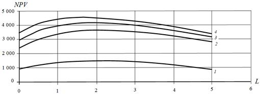
Fig. 2. Dependence of NPV on leverage L at t = 20% in 2010 year: 1 – for two-year income from investments; 2 – for five-year income from investments (the term hardware depreciation); 3 – for seven years of investment income; 4 – for ten years of investment income.
In the company's investment in 2010 equity capital accounted for 65 %, and debt - 35 %, i.e. the leverage level was equal to L = 0.54 . The term hardware depreciation, into establishment of which investment were done, was five years. Curve 2 (Fig. 2 ) corresponds to dependence of NPV on leverage level for the five-year project. Optimum NPV is achieved when L = 2. At this leverage level NPV = 3 624.5 million dollars.
The level leverage with which company "Nastcom Plus" has carried out its investment projects (L = 0.54), was lying far from optimum and provided NPV = 2.979.2 million dollars, that is approximately 645 million dollars less than optimal NPV value.
Since the equipment can be operated and after depreciation, one can estimate the NPV and for a more long-term perspective. For example, seven-year project the optimal leverage value is L = 2.0, when the NPV = 4,157.6 million dollars, that is for 562.8 million dollars more than non-optimal values of NPV = 3,594.8 million dollars, obtained by the company. For the ten-year project the optimal leverage level L = 1.5, with NPV = 4,509.1 million dollars, that is for 422.9 million dollars more than non-optimal values of NPV = 4, 086.2 million dollars, obtained by the company (Fig. 2, Tables 2–4).
Analysis of investments in 2011 year Using company's data, we compute the WACC, ke and NVP (Tables 5–7, Fig. 3).
Table 5. Weighted average cost of capital WACC in 2011 year.
| project duration n | Leverage level L | ||||||||||
| 0 | 0.5 | 1 | 1.5 | 2 | 2.5 | 3 | 3.5 | 4 | 4.5 | 5 | |
| 2 | 0.2367 | 0.3096 | 0.3824 | 0.4552 | 0.5280 | 0.6008 | 0.6736 | 0.7464 | 0.8192 | 0.8920 | 0.9649 |
| 5 | 0.2367 | 0.3063 | 0.3758 | 0.4452 | 0.5147 | 0.5841 | 0.6536 | 0.7230 | 0.7925 | 0.8619 | 0.9314 |
| 7 | 0.2367 | 0.3053 | 0.3738 | 0.4423 | 0.5107 | 0.5791 | 0.6480 | 0.7165 | 0.7850 | 0.8535 | 0.9220 |
| 10 | 0.2366 | 0.3044 | 0.3720 | 0.4396 | 0.5071 | 0.5746 | 0.6422 | 0.7097 | 0.7772 | 0.8447 | 0.9122 |
Table 6. Equity cost ke in 2011 year.
| project duration n | Leverage level L | ||||||||||
| 0 | 0.5 | 1 | 1.5 | 2 | 2.5 | 3 | 3.5 | 4 | 4.5 | 5 | |
| 2 | 0.2367 | 0.3142 | 0.3916 | 0.4690 | 0.5464 | 0.6239 | 0.7013 | 0.7787 | 0.8561 | 0.9335 | 1.0110 |
| 5 | 0.2367 | 0.3110 | 0.3853 | 0.4595 | 0.5338 | 0.6080 | 0.6822 | 0.7565 | 0.8307 | 0.9049 | 0.9791 |
| 7 | 0.2367 | 0.3100 | 0.3833 | 0.4565 | 0.5297 | 0.6029 | 0.6761 | 0.7493 | 0.8230 | 0.8963 | 0.9695 |
| 10 | 0.2366 | 0.3091 | 0.3813 | 0.4536 | 0.5258 | 0.5980 | 0.6702 | 0.7424 | 0.8146 | 0.8868 | 0.9589 |
Table 7. Net present value, NPV, of the company in 2011 year, million dollars.
| project duration n | Leverage level L | ||||||||||
| 0 | 0.5 | 1 | 1.5 | 2 | 2.5 | 3 | 3.5 | 4 | 4.5 | 5 | |
| 2 | 418.8 | 460.5 | 415.8 | 302.3 | 133.3 | –80.9 | –332.5 | –615.0 | –923.5 | –1 254.0 | –1 603.1 |
| 5 | 1 704.2 | 2 025.4 | 2 131.8 | 2 089.9 | 1 943.2 | 1 721.0 | 1 443.5 | 1124.7 | 774.8 | 400.9 | 8.5 |
| 7 | 2 203.4 | 2 558.0 | 2 650.5 | 2 576.1 | 2 392.2 | 2 134.4 | 1 825.6 | 1480.7 | 1 105.7 | 715.0 | 309.8 |
| 10 | 2 648.2 | 2 982.3 | 3 028.1 | 2 907.1 | 2 685.2 | 2 399.5 | 2 071.6 | 1715.0 | 1 338.0 | 946.0 | 542.9 |
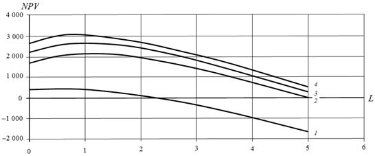
Fig. 3. Dependence of NPV on leverage L at t = 20% in 2011 year: 1 – for two-year income from investments; 2 – for five-year income from investments (the term hardware depreciation); 3 – for seven years of investment income; 4 – for ten years of investment income.
In the company's investment in 2011 equity capital accounted for 50 %, and debt capital - 50 % as well, i.e. the leverage level was equal to L = 1. The term hardware depreciation, into establishment of which investment were done, was five years. Curve 2 (Fig. 3) corresponds to dependence of NPV on leverage level for the five-year project. Optimum NPV is achieved approximately at L = 1. More accurate calculations show that optimal value NPV = 2,133.7 million dollars is achieved when L = 1.1.
The level leverage with which company "Nastcom Plus" has carried out its investment projects (L = 0.1), was lying in the vicinity of optimum and provided NPV = 2,131.8 million dollars, that is just 2 million dollars less than optimal NPV value. You can take it that, in 2011, investment in "Nastcom Plus" company have been carried out with almost optimal structure.
Analysis of investments in 2012 year Using company's data, we compute the WACC, ke and NVP (Tables 8–10, Fig. 4).
Table 8. Weighted average cost of capital WACC in 2012 year.
| project duration n | Leverage level L | ||||||||||
| 0 | 0.5 | 1 | 1.5 | 2 | 2.5 | 3 | 3.5 | 4 | 4.5 | 5 | |
| 2 | 0.2367 | 0.2298 | 0.2264 | 0.2243 | 0.2229 | 0.2219 | 0.2212 | 0.2206 | 0.2202 | 0.2198 | 0.2195 |
| 5 | 0.2367 | 0.2278 | 0.2234 | 0.2207 | 0.2189 | 0.2176 | 0.2167 | 0.2159 | 0.2153 | 0.2148 | 0.2144 |
| 7 | 0.2367 | 0.2272 | 0.2224 | 0.2195 | 0.2176 | 0.2162 | 0.2152 | 0.2143 | 0.2137 | 0.2132 | 0.2127 |
| 10 | 0.2366 | 0.2265 | 0.2213 | 0.2183 | 0.2162 | 0.2147 | 0.2136 | 0.2127 | 0.2120 | 0.2115 | 0.2110 |
Table 9. Equity cost ke in 2012 year.
| project duration n | Leverage level L | ||||||||||
| 0 | 0.5 | 1 | 1.5 | 2 | 2.5 | 3 | 3.5 | 4 | 4.5 | 5 | |
| 2 | 0.2367 | 0.3180 | 0.3992 | 0.4805 | 0.5617 | 0.6430 | 0.7242 | 0.8055 | 0.8867 | 0.9680 | 1.0492 |
| 5 | 0.2367 | 0.3150 | 0.3933 | 0.4715 | 0.5497 | 0.6279 | 0.7062 | 0.7844 | 0.8626 | 0.9408 | 1.0190 |
| 7 | 0.2367 | 0.3140 | 0.3913 | 0.4685 | 0.5457 | 0.6229 | 0.7001 | 0.7772 | 0.8544 | 0.9316 | 1.0088 |
| 10 | 0.2366 | 0.3130 | 0.3892 | 0.4653 | 0.5415 | 0.6177 | 0.6938 | 0.7699 | 0.8461 | 0.9222 | 0.9983 |
Table 10. Net present value NPV in 2012 year, million dollars.
| project duration n | Leverage level L | ||||||||||
| 0 | 0.5 | 1 | 1.5 | 2 | 2.5 | 3 | 3.5 | 4 | 4.5 | 5 | |
| 2 | 267.0 | 200.9 | 33.4 | –214.0 | –525.3 | –888.3 | –1 293.4 | –1 733.4 | –2 202.4 | –2 695.8 | –3 209.9 |
| 5 | 1 734.8 | 1 968.9 | 1 954.6 | 1 771.8 | 1 472.1 | 1 089.6 | 647.1 | 160.6 | –358.9 | –903.4 | –1 467.2 |
| 7 | 2 304.7 | 2 566.9 | 2 528.9 | 2 304.4 | 1 960.4 | 1 537.2 | 1 060.3 | 545.9 | 4.7 | –556.0 | –1 131.2 |
| 10 | 2 812.6 | 3 041.6 | 2 945.5 | 2 667.4 | 2 281.9 | 1 829.9 | 1 335.0 | 811.1 | 266.8 | –292.2 | –862.1 |
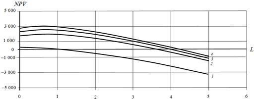
Fig. 4. Dependence of NPV on leverage L at t = 20% in 2012 year: 1 – for two-year income from investments; 2 – for five-year income from investments (the term hardware depreciation); 3 – for seven years of investment income; 4 – for ten years of investment income.
The company's investment structure in 2012 year was the same as in 2011: equity capital accounted for 50 %, and debt capital - for 50 %, i.e. the leverage level was equal to L =1. The term hardware depreciation, into establishment of which investment were done, was five years. Curve 2 (Fig. 4) corresponds to dependence of NPV on leverage level for the five-year project. Optimum NPV is achieved when L = 0.5. More accurate calculations show that optimal value NPV = 1. 987.7 million dollars is achieved when L = 0.7 (Table 11, Fig. 5).
Table 11. Net present value NPV at leverage level from 0.5 up to 1.05 in 2012 year, million dollars.
| project duration n | Leverage level L | |||||||||||
| 0.5 | 0.55 | 0.6 | 0.65 | 0.7 | 0.75 | 0.8 | 0.85 | 0.9 | 0.95 | 1 | 1.05 | |
| 2 | 200.9 | 188.3 | 174.8 | 160.2 | 144.8 | 128.4 | 111.1 | 92.9 | 73.9 | 54.1 | 33.4 | 12.0 |
| 5 | 1 968.9 | 1 977.0 | 1 982.8 | 1 986.3 | 1 987.7 | 1 987.0 | 1 984.2 | 1 979.5 | 1 973.0 | 1 964.6 | 1 954.6 | 1 942.8 |
| 7 | 2 566.9 | 2 574.2 | 2 578.8 | 2 580.6 | 2 580.0 | 2 576.9 | 2 571.5 | 2 563.9 | 2 554.2 | 2 542.5 | 2 528.9 | 2 513.5 |
| 10 | 3 041.6 | 3 043.5 | 3 042.4 | 3 038.5 | 3 032.0 | 3 023.1 | 3 011.7 | 2 998.2 | 2 982.6 | 2 965.0 | 2 945.5 | 2 924.3 |
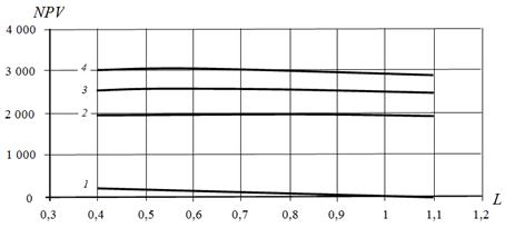
Fig. 5. Dependence of NPV on leverage L at t = 20% in 2012 year in the vicinity of optimum: 1 – for two-year income from investments; 2 – for five-year income from investments (the term hardware depreciation); 3 – for seven years of investment income; 4 – for ten years of investment income.
The level leverage, with which company "Nastcom Plus" has carried out its investment projects (L = 0.1 ), did not correspond to optimum value (L=0.7) and provided NPV = 1,954.6 million dollars, that is 31.7 million dollars less than optimal NPV value (Figs. 4 and 5 ; Tables 10 and 11).
Since the equipment can be operated and after depreciation, one can estimate the NPV and for a more long-term perspective. For example, for seven-year project the optimal leverage value is L =0.65, when the NPV = 2,580.6 million dollars, that is for 51.7 million dollars more than non-optimal values of NPV = 2,528.9 million dollars, obtained by the company. For the ten-year project the optimal leverage level L = 0.55, with NPV =3,043.5 million dollars , that is for 98 million dollars more than non-optimal values of NPV = 2,945.5 million dollars , obtained by the company.
2.2. The Dependence of NPV on the Equity Capital Value and Coefficient b
Let us investigate the dependence of NPV on the equity capital value and coefficient b (Tables 12–15, Figs. 6–9).
Table 12. Net present value NPV at β = 1.02, million dollars.
| Equity. S | Leverage level L | ||||||||||
| 0 | 0.5 | 1 | 1.5 | 2 | 2.5 | 3 | 3.5 | 4 | 4.5 | 5 | |
| 1 382 | 1 734.8 | 1 968.9 | 1 954.6 | 1 771.8 | 1 472.1 | 1 089.6 | 647.1 | 160.6 | –358.9 | –903.4 | –1 467.2 |
| 1 000 | 1 255.7 | 1 425.2 | 1 414.8 | 1 282.5 | 1 065.6 | 788.7 | 468.4 | 116.2 | –259.8 | –653.9 | –1 062.0 |
| 1 200 | 1 506.8 | 1 710.2 | 1 697.8 | 1539.0 | 1 278.7 | 946.4 | 562.1 | 139.5 | –311.8 | –784.7 | –1 274.4 |
| 1 600 | 2 009.1 | 2 280.3 | 2 263.7 | 2 052.0 | 1 705.0 | 1 261.9 | 749.5 | 186.0 | –415.7 | –1 046.3 | –1 699.2 |
| 1 800 | 2 260.3 | 2 565.3 | 2 546.7 | 2 308.5 | 1 918.1 | 1 419.7 | 843.2 | 209.2 | –467.6 | –1 177.1 | –1 911.6 |
Table 13. Net present value, NPV, at β = 0.5, million dollars.
| Equity. S | Leverage level L | ||||||||||
| 0 | 0.5 | 1 | 1.5 | 2 | 2.5 | 3 | 3.5 | 4 | 4.5 | 5 | |
| 1 382 | 146.1 | –71.8 | –411.5 | –833.8 | –1 313.3 | –1 833.5 | –2 383.1 | –2 954.2 | –3 541.6 | –4 141.1 | –4 750.2 |
| 1 000 | 105.7 | –52.0 | –297.9 | –603.5 | –950.7 | –1 327.2 | –1 725.0 | –2 138.4 | –2 563.6 | –2 997.6 | –3 438.4 |
| 1 200 | 126.9 | –62.4 | –357.4 | –724.2 | –1 140.8 | –1 592.6 | –2 070.0 | –2 566.1 | –3 076.3 | –3 597.1 | –4 126.1 |
| 1 600 | 169.2 | –83.2 | –476.6 | –965.6 | –1 521.0 | –2 123.5 | –2 760.0 | –3 421.5 | –4 101.7 | –4 796.1 | –5 501.4 |
| 1 800 | 190.3 | –93.6 | –536.2 | –1 086.3 | –1 711.2 | –2 388.9 | –3 105.0 | –3 849.2 | –4 614.4 | –5 395.6 | –6 189.1 |
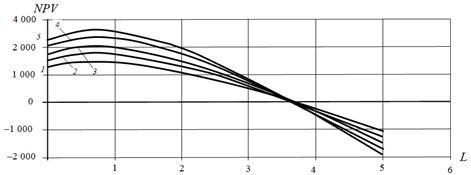
Fig. 6. Dependence of NPV on leverage at different values of equity cost S at b=1.02, million dollars: 1 – S = 1,382. 2 million dollars; 2 – S = 1 000 million dollars; 3 – S = 1 200 million dollars; 4 – S = 1 600 million dollars; 5 – S = 1 800 million dollars.
With increase of the equity value, optimum is observed for all of the values S when leverage level is approximately equal to L = 0.7, and the optimum value, as well as the NPV value is growing with increasing S, as long as the project remains effective (up to the leverage level approximately L = 3.7 ).
With decrease of the return on investment (b = 0.5) the dependence of the NPV on leverage changes significantly: now NPV monotonically decreases with the leverage at all values of equity capital S (Fig. 7 ).
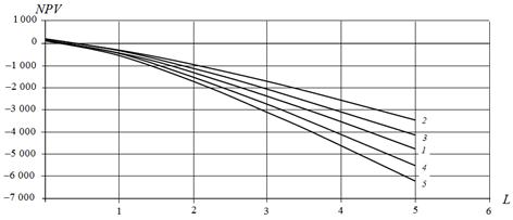
Fig. 7. Dependence of NPV on leverage at different values of equity cost S at b=0.5, million dollars: 1 – S = 1 382, 2 million dollars; 2 – S = 1 000 million dollars; 3 – S = 1 200 million dollars; 4 – S = 1 600 million dollars; 5 – S = 1 800 million dollars.
Table 14. Net present value NPV at β = 1.5, million dollars.
| Equity. S | Leverage level L | ||||||||||
| 0 | 0.5 | 1 | 1.5 | 2 | 2.5 | 3 | 3.5 | 4 | 4.5 | 5 | |
| 1 382 | 3 201.2 | 3 852.6 | 4 138.6 | 4 176.9 | 4 043.3 | 3 787.8 | 3 444.2 | 3 035.8 | 2 578.9 | 2 085.3 | 1 563.3 |
| 1 000 | 2 32 | 2 788.7 | 2 995.8 | 3 023.5 | 2 926.8 | 2 741.8 | 2 493.1 | 2 197.5 | 1 866.7 | 1 509.4 | 1 131.6 |
| 1 200 | 2 780.7 | 3 346.5 | 3 594.9 | 3 628.2 | 3 512.1 | 3 290.2 | 2 991.7 | 2 637.0 | 2 240.1 | 1 811.3 | 1 357.9 |
| 1 600 | 3 707.5 | 4 462.0 | 4 793.2 | 4 837.6 | 4 682.8 | 4 386.9 | 3 989.0 | 3 515.9 | 2 986.8 | 2 415.1 | 1 810.6 |
| 1 800 | 4 171.0 | 5 019.7 | 5 392.4 | 5 442.3 | 5 268.2 | 4 935.3 | 4 487.6 | 3 955.4 | 3 360.1 | 2 716.9 | 2 036.9 |
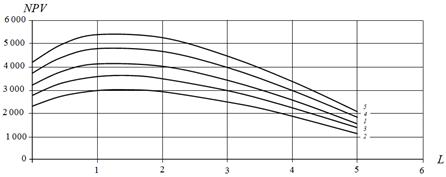
Fig. 8. Dependence of NPV on leverage at different values of equity cost S at b=1.5, million dollars: 1 – S = 1382. 2 million dollars; 2 – S = 1000 million dollars; 3 – S = 1200 million dollars; 4 – S = 1600 million dollars; 5 – S = 1800 million dollars.
With increase of the return on investment (b = 1.5) the NPV of the project has an optimum at all values of equity capital S at leverage level L=1.5 and NPV(L) curve is going up with the increase in S until the project remains effective (up to the leverage level approximately L = 7). The optimum position (value L0) is almost does not depend on the equity value S (L0 = 1.5). This means the possibility of a tabulation of obtained results by the known values k0 and kd for large values![]() , when in dependence of NPV(L) there is an optimum.
, when in dependence of NPV(L) there is an optimum.
Table 15. Net present value, NPV , at β = 2.0, million dollars.
| Equity. S | Leverage level L | ||||||||||
| 0 | 0.5 | 1 | 1.5 | 2 | 2.5 | 3 | 3.5 | 4 | 4.5 | 5 | |
| 1 382 | 4 728.8 | 5 814.9 | 6 413.7 | 6 682.3 | 6 721.7 | 6 598.5 | 6 357.9 | 6 030.8 | 5 639.2 | 5 198.5 | 4 720.0 |
| 1 000 | 3 423.0 | 4 209.1 | 4 642.6 | 4 837.0 | 4 865.5 | 4 776.3 | 4 602.2 | 4 365.4 | 4 081.9 | 3 762.9 | 3 416.6 |
| 1 200 | 4 107.5 | 5 050.9 | 5 571.1 | 5 804.4 | 5 838.6 | 5 731.6 | 5 522.6 | 5 238.5 | 4 898.3 | 4 515.5 | 4 099.9 |
| 1 600 | 5 476.7 | 6 734.5 | 7 428.1 | 7 739.2 | 7 784.8 | 7 642.1 | 7 363.4 | 6 984.7 | 6 531.1 | 6 020.6 | 5 466.6 |
| 1 800 | 6 161.3 | 7 576.4 | 8 356.6 | 8 706.6 | 8 757.9 | 8 597.4 | 8 283.9 | 7 857.8 | 7 347.4 | 6 773.2 | 6 149.9 |
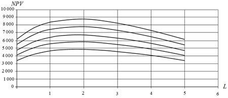
Fig. 9. Dependence of NPV on leverage at different values of equity cost S at b=2, million dollars: 1 – S = 1 382, 2 million dollars; 2 – S = 1 000 million dollars; 3 – S = 1 200 million dollars; 4 – S = 1 600 million dollars; 5 – S = 1 800 million dollars.
With further increase of the return on investment (b = 2) NPV of the project has an optimum for all values S at leverage level which is already approximately equal to L = 1.8, and the value of optimum as well as of NPV in general is growing with increasing S, until the project remains an effective (up to leverage level of order L=8.5, see Fig. 9).
In this way, the analysis of the dependence of NPV on the equity value S and on the return on investment b allows us conclude, that in contrast to the parameters I and NOI the change of parameters S and b, both individually and simultaneously, can significantly change the nature of the dependence of NPV on leverage level.
With increase of return on investment (with the increased b) there is a transition from the monotonic decrease of NPV of the project with leverage (Fig. 7 ) to the existing of the optimum at all values of S (see fig. 6 and 8 ). The growth of b leads to growth of NPV as well as to growth of the limit leverage value, up to which project remains an effective.
This means the inability of tabulation of the results, obtained in the general case of a constant value of equity capital: in this case, it is necessary to use the obtained by authors in the works (Brusov et al 2011a,b,c,d,e; 2012 a,b; 2013 a,b,c; 2014 a,b; Filatova et al 2008) formulas to determine the NPV at the existing leverage level, as well as for optimization of existing investment structure. Tabulation is possible only in the case of large b values (![]() ), when there is an optimum in the dependence of NPV on the leverage level.
), when there is an optimum in the dependence of NPV on the leverage level.
2.3. Conclusions
In 2010, the company "Nastcom Plus" worked at leverage level L = 0.54 instead of optimal value L = 2.0. The NPV loss amounted to 645 million dollars.
In 2012, the company worked at leverage level L = 1.0 instead of optimal value L = 0.7 . The NPV loss amounted from 32 to 98 million dollars, depending on the term of operation of equipment.
The authors have evaluated effectiveness of investment at existing level of debt financing and have developed recommendations on the optimum level of leverage for the Russian company "Nastcom Plus" in 2010-2012.
The results indicate that, if in 2011 financial structure of investment of company " Nastcom Plus" was close to the optimal and NPV was only 2 million dollars less than the optimal value, in 2010, when the leverage level was L = 0.54, NPV was 645 million dollars less than optimal value (the optimal leverage level should be equal to L = 2).
In 2012 the leverage level, with which company "Nastcom Plus" has carried out its investment projects (L = 0.1 ), did not correspond to optimum value (L=0.7) and provided NPV = 1,954.6 million dollars, that is 31.7 million dollars less than optimal NPV value (Tables 10 and 11; Figs. 4;5).
Since the equipment can be operated and after depreciation, one can estimate the NPV and for a more long-term perspective. For example, for seven-year project the optimal leverage value is L =0.65, when the NPV = 2,580.6 million dollars, that is for 51.7 million dollars more than non-optimal values of NPV = 2,528.9 million dollars, obtained by the company. For the ten-year project the optimal leverage level L = 0.55, with NPV =3,043.5 million dollars , that is for 98 million dollars more than non-optimal values of NPV = 2,945.5 million dollars , obtained by the company.
3. Effects of Taxation on the Optimal Capital Structure of Companies in the Telecommunication Sector
We continue the analysis of activity of the company "Nastcom Plus". In this paragraph we examine the effect of change of tax on profit rate, both in the case of its increase as well as decrease, on optimal structure of investments at different project durations.
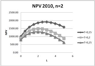
Fig. 10. Dependence of NPV on leverage level L for three values of tax on profit rate: T=15%;20%;25% for two-year project in 2010.
It is shown, that increasing of tax on profit rate leads to degradation (decreasing) of NPV, and degradation is reduced with an increase project duration. In particular, for the five-year project (amortization period) when the tax on profit rate decreases on 1%, NPV decreases on 1.5% - 2.34% in different years.
Impact of change of tax on the profit rate on the optimum position while it exists (change optimum position is changed for two-years and ten-years projects in 2010, and for the five-year project in the 2012 year (for 0.5 -1 (in L units)), nevertheless the optimum position turns out to be sufficiently stable.
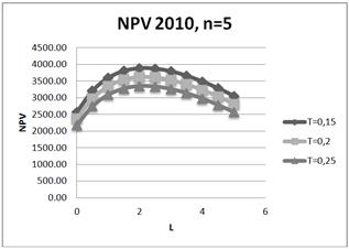
Fig. 11. Dependence of NPV on leverage level L for three values of tax on profit rate: T=15%;20%;25% for five-year project in 2010.
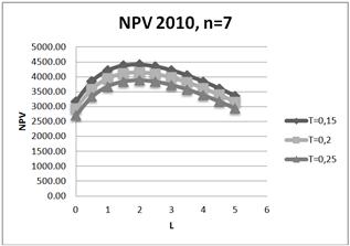
Fig. 12. Dependence of NPV on leverage level L for three values of tax on profit rate: T=15%;20%;25% for seven-year project in 2010.
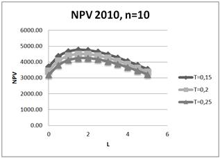
Fig. 13. Dependence of NPV on leverage level L for three values of tax on profit rate: T=15%;20%;25% for ten-year project in 2010.
Table 16. Dependence of optimum position of investment structure in 2010 on tax on profit rate and project duration.
| 2010 t\n | 2 | 5 | 7 | 10 |
| 15% | 3 | 2 | 2 | 2 |
| 20% | 2 | 2 | 2 | 1.5 |
| 25% | 2 | 2 | 2 | 2 |
Table 17. Absolute and relative change of NPV with increase/decrease of tax on profit rate on 5% (1%) in 2010.
| 2010 | t=20%-15% | t=25%-20% | On 5% | On 1% |
| n=2 | 418/487 | 204 | 34% | 6.8% |
| 5 | 266 | 273 | 7.45% | 1.49% |
| 7 | 263 | 271 | 6.88% | 1.37% |
| 10 | 245 | 256 | 5. 56% | 1.11% |
Table 18. Dependence of optimum position of investment structure in 2011 on tax on profit rate and project duration.
| 2011 t\n | 2 | 5 | 7 | 10 |
| 15% | 0.5 | 1 | 1 | 1 |
| 20% | 0.5 | 1 | 1 | 1 |
| 25% | 0.5 | 1 | 1 | 1 |
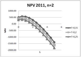
Fig. 14. Dependence of NPV on leverage level L for three values of tax on profit rate: T=15%;20%;25% for two-year project in 2011.
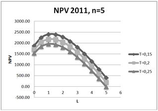
Fig. 15. Dependence of NPV on leverage level L for three values of tax on profit rate: T=15%;20%;25% for five-year project in 2011.
Table 19. Absolute and relative change of NPV with increase/decrease of tax on profit rate on 5% (1%) in 2011.
| 2011 | t=20%-15% | t=25%-20% | On 5% | On 1% |
| n=2 | 119 | 118 | 25.8% | 5.16% |
| 5 | 222 | 223 | 10.2% | 2.04% |
| 7 | 236 | 239 | 8.75% | 1.75% |
| 10 | 238 | 242 | 7.7% | 1.54% |
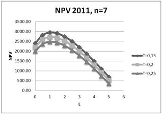
Fig. 16. Dependence of NPV on leverage level L for three values of tax on profit rate: T=15%;20%;25% for seven-year project in 2011.
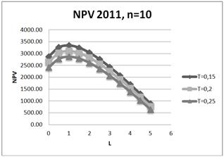
Fig. 17. Dependence of NPV on leverage level L for three values of tax on profit rate: T=15%;20%;25% for ten-year project in 2011.
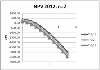
Fig. 18. Dependence of NPV on leverage level L for three values of tax on profit rate: T=15%;20%;25% for two-year project in 2012.
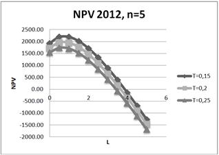
Fig. 19. Dependence of NPV on leverage level L for three values of tax on profit rate: T=15%;20%;25% for five-year project in 2012.
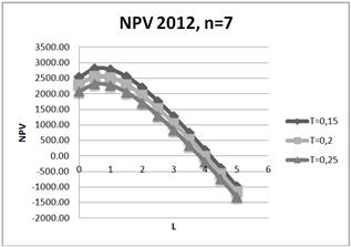
Fig. 20. Dependence of NPV on leverage level L for three values of tax on profit rate: T=15%;20%;25% for seven-year project in 2012.
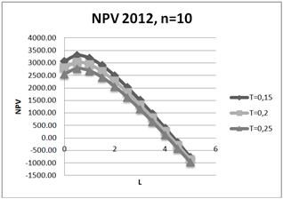
Fig. 21. Dependence of NPV on leverage level L for three values of tax on profit rate: T=15%;20%;25% for ten-year project in 2012.
Table 20. Dependence of optimum position of investment structure in 2010 on tax on profit rate and project duration.
| 2012 t\n | 2 | 5 | 7 | 10 |
| 15% | 0 | 1 | 0.5 | 0.5 |
| 20% | 0 | 0.5 | 0.5 | 0.5 |
| 25% | 0 | 0.5 | 0.5 | 0.5 |
Table 21. Absolute and relative change of NPV with increase/decrease of tax on profit rate on 5% (1%) in 2012.
| 2012 | t=20%-15% | t=25%-20% | On 5% | On 1% |
| n=2 | 104 | 103 | 39% | 7.8% |
| 5 | 229 | 229 | 11.7% | 2.34% |
| 7 | 253 | 256 | 9.9% | 1.98% |
| 10 | 269 | 271 | 8.9% | 1.74% |
It is shown, that increasing of tax on profit rate leads to degradation (decreasing) of NPV, and degradation is reduced with an increase of project duration. Note, that for the five-year project (amortization period) when the tax on profit rate decreases on 1%, NPV decreases on 2.34% in 2012, on 2.04% - in 2011 and on 1.49 - in 2010.
4. Conclusions
Paper is devoted to optimizing of the investment structure of the telecommunication sector company "Nastcom Plus". We examine the effect of change of tax on profit rates, both in the case of its increase as well as decrease, on optimal structure of investments at different project durations. All calculations have been done within modern theory of capital cost and capital structure by Brusov-Filatova-Orekhova. The analysis of investments carried out by the formula, obtained by us earlier for the case of constant value of equity capital. Consideration has been done from the point of view of owners of equity capital.
It is shown that increasing of tax on profit rates leads to degradation (decreasing) of NPV, and degradation is reduced with an increase project duration. In particular, for 5-year project (amortization period) with increase of tax on profit rate on 1% NPV decreases on 1,5%-2,34% for different years.
Influence of change of tax on profit rate, while there is, (optimum for 2-years and 10-years projects in 2012 is changed (on 0,5-1 (in leverage units)), nevertheless the optimum position is stable
References
- Brusov P, Filatova T, Orehova N, Eskindarov M (2015), Modern corporate finance, investments and taxation, Springer International Publishing, Switzerland, 373 p.
- Brusov P, Filatova T, Orehova N, Brusova A (2011a) Weighted average cost of capital in the theory of Modigliani–Miller, modified for a finite life–time company. Applied Financial Economics 21(11): 815-824
- Brusov P, Filatova P, Orekhova N (2013a) Absence of an Optimal Capital Structure in the Famous Tradeoff Theory! Journal of Reviews on Global Economics 2: 94-116
- Brusov P, Filatova P, Orekhova N (2014a) Mechanism of formation of the company optimal capital structure, different from suggested by trade off theory. Cogent Economics & Finance 2: 1-13 http://dx.doi.org/10.1080/23322039.2014.946150
- Brusov P, Filatova T, Orehova N et al. (2011b) From Modigliani–Miller to general theory of capital cost and capital structure of the company. Research Journal of Economics, Business and ICT 2: 16–21
- Brusov P, Filatova T, Eskindarov M, Orehova N (2012a) Influence of debt financing on the effectiveness of the finite duration investment project. Applied Financial Economics 22 (13) : 1043-1052
- Brusov P, Filatova T, Orehova N et al (2011c) Influence of debt financing on the effectiveness of the investment project within the Modigliani–Miller theory. Research Journal of Economics, Business and ICT (UK) 2: 11-15
- Brusov P, Filatova T, Eskindarov M, Orehova N (2012b) Hidden global causes of the global financial crisis. Journal of Reviews on Global Economics 1: 106-111
- Brusov P, Filatova T, Orekhova N (2013b) Absence of an Optimal Capital Structure in the Famous Tradeoff Theory! Journal of Reviews on Global Economics 2: 94–116
- Brusov P.N., Filatova Т. V. (2011d) From Modigliani–Miller to general theory of capital cost and capital structure of the company. Finance and credit 435: 2–8.
- Brusov P Filatova T Orehova N Brusov P.P Brusova N. (2011e) From Modigliani–Miller to general theory of capital cost and capital structure of the company. Research Journal of Economics, Business and ICT 2: 16–21
- Brusov P Filatova T Orehova N (2014b) Inflation in Brusov–Filatova–Orekhova Theory and in its Perpetuity Limit – Modigliani – Miller Theory.Journal of Reviews on Global Economics 3: 175-185
- Brusov P Filatova T Orehova N (2013c) A Qualitatively New Effect in Corporative Finance: Abnormal Dependence of Cost of Equity of Company on Leverage. Journal of Reviews on Global Economics 2: 183-193
- Filatova Т Orehova N Brusova А (2008) Weighted average cost of capital in the theory of Modigliani–Miller, modified for a finite life–time company. Bulletin of the FU 48: 68–77
- Brusova A (2011) А Comparison of the three methods of estimation of weighted average cost of capital and equity cost of company. Financial analysis: problems and solutions 34 (76): 36-42
- Мodigliani F, Мiller M (1958) The Cost of Capital, Corporate Finance, and the Theory of Investment. American Economic Review 48: 261–297
- Мodigliani F, Мiller M (1963) Corporate Income Taxes and the Cost of Capital: A Correction. American Economic Review 53: 147–175
- Modigliani F, Miller M (1966) Some estimates of the Cost of Capital to the Electric Utility Industry 1954–1957 . American Economic Review 56: 333-391


