
International Journal of Modern Physics and Applications, Vol. 1, No. 3, July 2015 Publish Date: Jun. 24, 2015 Pages: 64-72
Embedding Dimension as Input Dimension of Artificial Neural Network: A Study on Stock Prices Time Series
Amir Hosein Ghaderi1, *, Bahar Barani2, Hoda Jalalkamali1
1Neuroscience Lab., University of Tabriz, Tabriz, Iran
2Medical School, University of Kansas, Kansas City, USA
Abstract
Recently artificial neural networks (ANNs) have become crucial for the analysis of several phenomena in the world. Stock market prices is a nonlinear phenomenon that several studies are accomplished in this context using ANN. Determine the input dimension of network is a basic problem in application of ANN to prediction of stock prices. On the other hand, stock market behaves as a chaotic system with nonlinear and deterministic manner. Therefore chaos theory can be helpful to determine the input dimension of network. In this study a multilayer perceptron with Backpropagation learning algorithm is used for forecasting of stock prices in Tehran Stock Exchange (TSE). Prediction accuracy of ANN with various input dimensions is compared and the best result is achieved when the input dimension is equal to Takens embedding dimension. It is concluded that selection of Takens embedding as ANN input dimension can be led to very accurate predictions and best results in TSE.
Keywords
Neural Network, Chaos Theory, Multilayer Perceptron, Embedding Dimension, Stock Market, Forecasting
Received: April 13, 2015
Accepted: April 20, 2015
Published online: June 23, 2015
@ 2015 The Authors. Published by American Institute of Science. This Open Access article is under the CC BY-NC license. http://creativecommons.org/licenses/by-nc/4.0/
1. Introduction
Overall, there are several nonlinear phenomena across the world. The change in climate, the activity of the mammalian brain, the social behavior of humans, the probability of an earthquake occurring, and the fluctuating prices in the stock market are just a few examples of nonlinearity in the world. Recently, several methods have been suggested for the prediction of these nonlinear phenomena and therefore, the analysis and prediction of these has become a vital tool to the advancement of science. Chaotic and fractal analysis, time series analysis, the genetic algorithm, fuzzy logic, and neural networks are continually being extended for a nonlinear world analysis.
Upon a first glance at the fluctuations of the prices of stock, it seems that there is no pattern or order to the fluctuations. However, in numerous studies, it has been shown that these fluctuations do in fact follow a specific order. Some of the studies show that this behavior is chaotic and deterministic, therefore making the prediction of these fluctuations possible [1–3]. Recently, nonlinear analysis has become crucial for the analysis of price fluctuations in the stock market. SVR [4–6], fuzzy logic, genetic algorithm [8,9] and neuro fuzzy [10,11] are some of these nonlinear approaches and have shown that fluctuations of the prices of stock can be predicted.
One of the well-known approaches to the prediction of time series changes is the artificial neural network method [12–14]. Artificial neural network (ANN) is a reliable model for classification and prediction in many areas such as signal processing, aerology, motor control and thermodynamics and so on. Many studies suggest this model for stock analysis. In decade of 1990 ANN was used for price forecasting and showed its superiority over the linear models such as ARIMA [18–20]. Kohzadi et al. show that the neural network approach was able to prediction of wheat and cattle price, while the ARIMA approach was only able to do so for wheat. After wards various types of the artificial neural networks were employed to stock market forecasting. The multi layers perceptrons (MLPs) and back-propagation learning algorithm are used in many studies for stock price forecasting [21–23]. F. Castiglione shows that MLP able to forecast the sign of the price increments with a success rate slightly above 50% but he do not have a mechanism to find it with high probability. Q. Cao et al. use a feedforward neural network with one hidden layer for Chinese stock price prediction and indicate feedforward neural network is a useful tool for stock price forecasting in emerging markets, such as China. Other studies use recurrent networks rather than feedforward networks [25–27]. In recent years, several studies have been accomplished to improve network learning. The genetic algorithm has been used repeatedly as network learning algorithm in stock price applications [28–30]. Y. Zhang and L. Wu proposed a bacterial chemotaxis optimization (IBCO), which is then integrated into the BP algorithm for stock market prediction. They found that, this method show better performance than other methods in learning ability and generalization. W. Shen et al. used a radial basis function neural network (RBFNN) to train data and forecast the stock indices of the Shanghai Stock Exchange. They compared forecasting result of radial basis function optimized by several methods. Finally they found that RBF optimized by AFSA is an easy-to-use algorithm with considerable accuracy. A recurrent neural network (RNN) based on Artificial Bee Colony (ABC) algorithm was used by T.J. Hsieh et al. for stock markets forecasting. They used Artificial Bee Colony algorithm (ABC) to optimize the RNN weights. C.J. Lua and J.Y. Wu employed a cerebellar model articulation controller neural network (CAMC NN) for stock index forecasting to improve the forecasting performance. The forecasting results were compared with a support vector regression (SVR) and a back-propagation neural network (BPNN) and experimental results show that performance of the proposed CMAC NN scheme was superior to the SVR and BPNN models. An integrated approach based on genetic fuzzy systems (GFS) and ANN for constructing a stock price forecasting expert system is presented by E. Hadavandi et al. and they show that the proposed method is a suitable approach for stock price forecasting.
But, one of the problems that arise with the use of the supervisor learning ANN in time series analysis, such as the fluctuations in stock prices, is the specification of the input pattern dimension. In most studies, there is no specific rule in place for the specification of the input pattern dimension and the selection of this dimension has been accomplished experimentally [23,24,26,28]. F. Castiglione stated that there is no way to determine input and hidden units and N. Khoa et al. represented that network inputs, were decided based on experimental results.
On the other hand, in chaotic analysis the correlation dimension and the embedding dimension of a time series signal can be determined. If it is assumed that the price fluctuations in the stock market are a chaotic time series signal [1–3], then the chaotic analysis can be used to determine the correlation dimension and the embedding dimension of stock market price in time series. Z. Shang et al. have demonstrated that the employment of the embedding dimension as the input pattern dimension can lead to an appropriate result in a feedforward neural network method. They have shown that, in the chaotic maps, the input pattern dimension in the neural network must be equal to the embedding dimension. However, the embedding dimension can be found through the use of two different methods: the Grassberger method and the Takens method [37,38] and these two embedding dimensions have very different values in the chaotic analysis of the fluctuating prices of the stock market. O.J Kyong and K. Kyoung-jae show that embedding dimension can be used for determination of time lag size in input variable of ANN and they use Grassberger embedding dimension in stock price time series as input dimension for ANN learning.
In this work the first goal is to obtain a highly accurate method for the forecasting of the price of Iranian stock within short interval of time by a multi-layer perceptron ANN. The second objective mainly focuses on the application of chaotic analysis in order to determine the ANN input dimension. And lastly, in more detail, the second goal is to utilize a new approach in order to determine whether Grassberger embedding or Takens embedding is most useful in the determination of ANN input dimension in a given real-life application, such as stock market price fluctuations.
This paper is organized as follows; the chaotic analysis on time series and embedding dimension is described in section 2, the multilayer perceptrons and back-propagation learning algorithm is displayed in section 3, section 4 is devoted to the application of the embedding dimension for the determination of the neural network input dimension, and finally sections 5 and 6 are dedicated to the discussion and conclusion.
2. The Chaotic Dimensions
2.1. Correlation Dimension
Dynamical chaotic systems have a strange attractor in phase space. Strange attractor characterized by a correlation dimension Dcor. This component is smaller than number of degrees of freedom F, Dcor < F. In a long-time series, correlation dimension is achieved by considering correlation between time series points. For calculation of correlation dimension, the correlation integral should be determined. The correlation integral is defined by:
![]()
Where H(x) is Heaviside function, xi is position of i’th point in time series, r is radial distance around each reference point xi and T is time series length and ||…||denotes Euclidean norm. Then, the correlation dimension can be obtained by:
![]()
2.2. Embedding Dimension
In 1981 Takens presented a dimension for a chaotic attractor phase space and then this dimension nominated Takens embedding dimension. Takens asserted that in the turbulence attractors, this dimension can be used as phase space dimension. Embedding dimension can be used as a measure of independent variables of the system. Takens states that embedding dimension should be obtained by correlation dimension in a way that m ≥ 2Dcor + 1. This embedding dimension is also called full embedding dimension. On the other hand, in 1983 Grassberger and Procaccia suggested embedding dimension in a different overview. They calculated correlation dimension versus different values of embedding dimension of the attractor and defined minimum embedding dimension as n+1 that n is the point where correlation dimension saturates.
3. Multilayer Perceptron and Backpropagation Algorithm
In a feedforward ANN, the signals, fellow directly from input neurons to output layer. A multilayer feedforward neural network is constructed when some hidden layers are located between input and output layers. Layered architectures are those in which the set of computing units (neurons) in input layer only connected with neurons in first hidden layer and so on. Multilayer perceptrons or MLPs is termed to feedforward multilayer networks with sigmoid nonlinearities. In the MLP, the output of each neuron is:
![]() ,
,
where xi is input signal, ω is synaptic weight of neuron k and sig is a sigmoid function.
There are some algorithms for MLPs training. A most popular of these training algorithms is Back-propagation algorithm. In this algorithm, there are three stages for training: the feedforward of the input training pattern, the calculation of associated error and back-propagated error signal, and the improvement of the synaptic weights. The error signal at iteration n and at the output of neuron j is obtained by:
![]()
4. Application of Chaos Theory in Ann Input Dimension
The analysis is accomplished on the stocks of two corporations in Tehran Stock Exchange (TSE), Pars oil and Iran Transfo. All data are obtained from TSE at http:/www.irbourse.com/en/stats.aspx. The data is related to daily exchange stock price of these corporations from March 1995 to May 2013 and used for training (90%) and testing (10%). For price forecasting, the data is divided into time lag windows and each window can be used for forecasting the next day price. This is illustrated schematically in Fig. 1.
A multilayer perceptron with two hidden layers is used for forecasting. There are 20 neurons in each hidden layer and one neuron in output layer. The number of input neurons is related to time lag window. The architecture of the ANN is shown in Fig. 2. The trainrp algorithm is used for network training in MATLAB. trainrp is a network training function that updates weight and bias values according to the resilient back-propagation algorithm. Additional data about ANN is represented in Tab. 1.
Table 1. Additional data about ANN structure.
| Learning rate | Act. func. (hidden layer) | Act. func. (output layer) | Training algorithm | Epochs |
| 0.05 | tansig | logsig | trainrp | 50000 |
The correlation dimension and embedding dimension are calculated for each time series. These values are shown in Tab. 2. In this table embedding dimension is calculated in two ways. Takens embedding dimension is achieved by the first integer above 2Dcor+1 where Dcor is correlation dimension and Grassberger embedding dimension is obtained according to Fig. 3, 4. The performance of each input dimension is shown in Tab. 4, 3. The best performances of ANN forecasting with three neurons in input layer are shown in Fig. 5, 7 for two time series and the regressions of predicted prices are shown in Fig. 6, 8 for best and worst results.
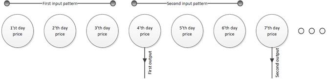
Figure 1. Determining the input dimension of ANN based on the time lag window.
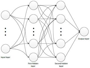
Figure 2. The architecture of an ANN with two hidden layers.
Table 2. Chaotic dimensions for two corporations’ time series.
| Corporation | Correlation dimension | Takens Em. dimension | Grassberger Em. dimension |
| Pars oil | 0.54 | 3 | 21 |
| Iran Transfo | 0.53 | 3 | 20 |
5. Discussion
The neural network input data is a critical matter in ANN training. The results show that various input size of ANN can be led to different accuracy of prediction. The importance of patterns input dimension in accuracy of prediction is demonstrated in Tab. 4, 3 and Fig. 6, 8. Fig. 8 indicates that there is a very little difference between input sizes of training patterns for best and worst predictions and Fig. 6 shows that selection of wrong input dimension can be led to false predictions. Therefore it is essential to determine input dimension of ANN, correctly.
The correlation dimension and the embedding dimension determine the properties of the phase space and attractor dimensions of the time series. Embedding dimension is equal to the number of independent variables of the system . On the other hand, the number of inputs of ANN and independent variables are identical, it seems that embedding dimension could be used for determining the input dimension of ANN.
In Oh and Kim study the Grassberger embedding dimension is used to determine the input dimension of ANN for stocks prices forecasting but they did not test performance of other input dimensions. Therefore in this study all input dimensions are tested and the results show that best prediction is achieved when the Takens embedding is selected as input dimension. Table 2 indicates that there is a large difference between Grassberger embedding and Takens embedding. In the Iranian stock market, Grassberger embedding is approximately 20, while Takens embedding is approximately 3. Choosing Takens’ embedding dimension leads to reliable results which are shown in Fig. 5, 7. These results suggest a new way to determine of the input size in ANN training.
Table 3. The performance results of Iran Transfo for various input dimensions.
| Input size | No. training patterns | No. testing patterns | R value | MSE | MAE |
| 2 | 793 | 88 | 0.75994 | 0.0000695 | 0.0066 |
| 3 | 528 | 58 | 0.97310 | 0.0000028 | 0.0014 |
| 4 | 396 | 44 | 0.97196 | 0.0000078 | 0.0024 |
| 5 | 316 | 35 | 0.94881 | 0.0000430 | 0.0060 |
| 6 | 263 | 29 | 0.97018 | 0.0000776 | 0.0084 |
| 7 | 225 | 25 | 0.94958 | 0.0001269 | 0.0108 |
| 8 | 197 | 21 | 0.93333 | 0.0000087 | 0.0024 |
| 9 | 175 | 19 | 0.95837 | 0.0002840 | 0.0164 |
| 10 | 157 | 17 | 0.71911 | 0.0003745 | 0.0183 |
| 11 | 143 | 16 | 0.94363 | 0.0000854 | 0.0086 |
| 12 | 131 | 15 | 0.86578 | 0.0003035 | 0.0170 |
| 13 | 121 | 13 | 0.95720 | 0.0001783 | 0.0127 |
| 14 | 112 | 13 | 0.77959 | 0.0005682 | 0.0231 |
| 15 | 104 | 11 | 0.90818 | 0.0006931 | 0.0256 |
| 16 | 98 | 11 | 0.94048 | 0.0000471 | 0.0064 |
| 17 | 92 | 10 | 0.68281 | 0.0003585 | 0.0177 |
| 18 | 87 | 10 | 0.73465 | 0.0001222 | 0.0102 |
| 19 | 82 | 9 | 0.53883 | 0.0002304 | 0.0134 |
| 20 | 78 | 9 | 0.90877 | 0.0000650 | 0.0075 |
Table 4. The performance results of Pars Oil for various input dimensions.
| Input size | No. training patterns | No. testing patterns | R value | MSE | MAE |
| 2 | 1354 | 151 | 0.95822 | 0.0001177 | 0.0027 |
| 3 | 906 | 101 | 0.99654 | 0.0000063 | 0.0018 |
| 4 | 679 | 76 | 0.84597 | 0.0002768 | 0.0040 |
| 5 | 543 | 60 | 0.99491 | 0.0000082 | 0.0021 |
| 6 | 452 | 50 | 0.99552 | 0.0000089 | 0.0025 |
| 7 | 387 | 43 | 0.98076 | 0.0000352 | 0.0043 |
| 8 | 339 | 38 | 0.99612 | 0.0000066 | 0.0018 |
| 9 | 301 | 34 | 0.99351 | 0.0000105 | 0.0024 |
| 10 | 271 | 30 | 0.99484 | 0.0000082 | 0.0023 |
| 11 | 246 | 27 | 0.97164 | 0.0000452 | 0.0046 |
| 12 | 225 | 25 | 0.99447 | 0.0000109 | 0.0028 |
| 13 | 208 | 23 | 0.98709 | 0.0000212 | 0.0034 |
| 14 | 193 | 22 | 0.99361 | 0.0000138 | 0.0030 |
| 15 | 180 | 20 | 0.99414 | 0.0000077 | 0.0022 |
| 16 | 169 | 19 | 0.98822 | 0.0000216 | 0.0037 |
| 17 | 159 | 17 | 0.99374 | 0.0000175 | 0.0031 |
| 18 | 150 | 17 | 0.99438 | 0.0000165 | 0.0033 |
| 19 | 142 | 16 | 0.99563 | 0.0000069 | 0.0020 |
| 20 | 135 | 15 | 0.99140 | 0.0000164 | 0.0032 |
| 21 | 128 | 14 | 0.98468 | 0.0000281 | 0.0043 |
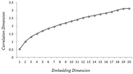
Figure 3. Grassberger embedding for Iran Transfo time series.
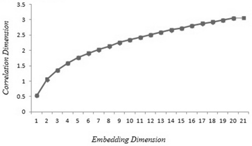
Figure 4. Grassberger embedding for Pars Oil time series.
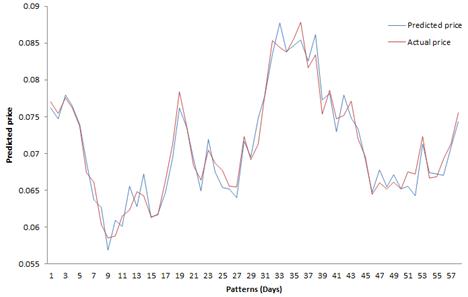
Figure 5. Comparison between predicted and actual data for Iran Transfo with Takens embedding input dimension.
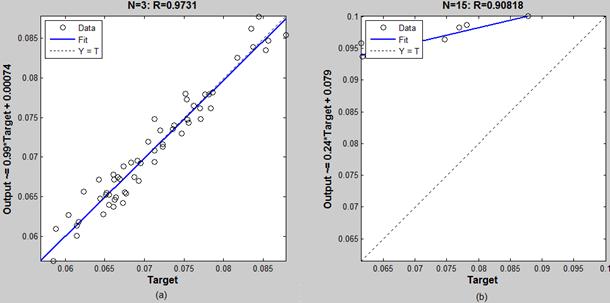
Figure 6. The best and worst regressions of ANN for Iran Transfo predicted price. a) Best result: 3 neurons in input layer. b) Worst result: 15 neurons in input layer.
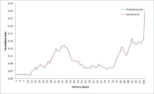
Figure 7. Comparison between predicted and actual data for Pars Oil with Takens embedding input dimension.
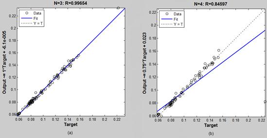
Figure 8. The best and worst regressions of ANN for Pars Oil predicted price. a) Best result: 3 neurons in input layer. b) Worst result: 4 neurons in input layer.
6. Conclusion
The results show that best performance of stock price forecasting is achieved when ANN input dimension is selected equal to Takens’ embedding dimension. This result is satisfied for both Iran Transfo (MSE=0.0000028) and Pars Oil (MSE=0.0000063) corporations as indicated in Tab 4, 3. Finally we found that good predicts could be performed in TSE using an ANN when input dimension is chosen based on the Takens’ embedding dimension. The reliability of these predictions is shown in Fig. 5, 7. Therefore, we suggest that Takens’ embedding dimension could be used in other time series predications with ANN.
References
- Peters EE. A chaotic attractor for the SP 500. Financial Analysts Journal, 1991:55-81.
- Qian B, Rasheed K. Stock market prediction with multiple classifiers. Applied Intelligence 2007;26 (1):25-33.
- Shively PA. The nonlinear dynamics of stock prices. The Quarterly Review of Economics and Finance 2003; 43 (3):505-17.
- Huang SC, Chuang PJ, Wu CF, Lai HJ. Chaos-based support vector regressions for exchange rate forecasting. Expert Systems with Applications 2010; 37(12):8590-98.
- Kao LJ, Chiu CC, Lu CJ, Yang JL. Integration of nonlinear independent component analysis and support vector regression for stock price forecasting. Neurocomputing. 2013; 99:53442.
- Kazem A, Sharifi E, Hussain FK, Saberi M, Hussain OK. Support vector regression with chaos-based firefly algorithm for stock market price forecasting. Applied Soft Computing 2013; 13: 94758.
- Wang YF. Predicting stock price using fuzzy grey prediction system. Exspert Systems with Applications 2002; 22(1):33-38.
- Naik RL, Ramesh D, Manjula B, Govardhan A. Prediction of Stock Market Index Using Genetic Algorithm. Computer Engineering and Intelligent Systems 2012; 3(7):162-71.
- Shaverdi M, Fallahi S, Bashiri V. Prediction of Stock Price of Iranian Petrochemical Industry Using GMDH-Type Neural Network andGenetic algorithm. Applied Mathematical Sciences 2012; 6(7):319-32.
- Esfahanipour A, Aghamiri W. Adapted neuro-fuzzy inference system on indirect approach TSK fuzzy rule base for stock market analysis. Expert Systems with Applications 2010; 37(7):4742-48.
- Liu CF, Yeh CY, Lee SJ. Application of type-2 neuro-fuzzy modeling in stock price prediction. Applied Soft Computing, 2012; 12(4):1348-58.
- Ghaderi AH, Darooneh AH. ARTIFICIAL NEURAL NETWORK WITH REGULAR GRAPH FOR MAXIMUM AIR TEMPERATURE FORECASTING: THE EFFECT OF DECREASE IN NODES DEGREE ON LEARNING. International Journal of Modern Physics C 2012; 23 (02):1-10.
- Zhang GP. Time series forecasting using a hybrid ARIMA and neural network model. Neurocomputing 2003; 50: 159-75.
- Ardalani-Farsa M, Zolfaghari S. Chaotic time series prediction with residual analysis method using hybrid Elman-NARX neural networks. Neurocomputing 2010; 73(13):2540-53.
- Hen HY, Hwang JN. Handbook of neural network signal processing. CRC press, 2010.
- Senjyu T, Miyazato H, Yokoda S, Uezato K. Speed control of ultrasonic motors using neural network. Power Electronics, IEEE Transactions on 1998;13(3):381-87.
- Ghaderi F. Ghaderi AH, Najafi B, Ghaderi N. Viscosity Prediction by Computational Method and Artificial Neural Network Approach: The Case of Six Refrigerants. The Journal of Supercritical Fluids 2013; 81: 6778.
- Kohzadi N, Boyd MS, Kermanshahi B, Kaastra I. A comparison of artificial neural network and time series models for forecasting commodity prices. Neurocomputing 1996; 10 (2):169-81.
- Wood D, Dasgupta B. Classifying trend movements in the MSCI USA capital market indexa comparison of regression, ARIMA and neural network methods. Computers Operations Research 1996; 23 (6):611-22.
- Yao J, Tan CL, Poh HL. Neural networks for technical analysis: a study on KLCI. International journal of theoretical and applied finance 1999:2(02):221-41. 9.
- Kaastra I, Boyd M. Designing a neural network for forecasting financial and economic time series. Neurocomputing 1996; 10(3):215-36.
- Huang W, Lai KK, Nakamori Y, Wang S, Yu L. Neural networks in finance and economics forecasting. International Journal of Information Technology Decision Making 2007; 6 (01):113-40.
- Castiglione F. Forecasting price increments using an artificial Neural Network. Advances in Complex Systems 2001;4(01):45-56
- Cao Q, Leggio KB, Schniederjans MJ. A comparison between Fama and French’s model and artificial neural networks in predicting theChinese stock market. Computers Operations Research 2005; 32 (10):2499-512.
- Roman J, Jameel A. (1996, January). Backpropagation and recurrent neural networks in financial analysis of multiple stock market returns. In System Sciences, 1996, Proceedings of the Twenty-Ninth Hawaii International Conference on, IEEE (Vol. 2, pp. 454-460).
- Khoa NLD, Sakakibara K, Nishikawa I. Stock price forecasting using back propagation neural networks with time and profit based adjusted weight factors. In SICE-ICASE International Joint Conference, IEEE 2006 (pp. 5484-5488).
- Wah BenjaminW, Minglun Qian. "Constrained formulations and algorithms for stock-price predictions using recurrent FIR neural networks." PROCEEDINGS OF THE NATIONAL CONFERENCE ON ARTIFICIAL INTELLIGENCE. Menlo Park, CA; Cambridge, MA; London; AAAI Press; MIT Press; 1999, 2002.
- Kim KJ, Han I. Genetic algorithms approach to feature discretization in artificial neural networks for the prediction of stock price index. Expert systems with applications 2000; 19 (2):125-32.
- Leigh W, Purvis R, Ragusa JM. Forecasting the NYSE composite index with technical analysis, pattern recognizer, neural network, andgenetic algorithm: a case study in¡ i¿ romantic¡/i¿ decision support. Decision Support Systems 2002; 32 (4):361-77.
- Du P, Luo X, He Z, Xie L. The application of genetic algorithm-radial basis function (ga-rbf) neural network in stock forecasting. In Control and Decision Conference (CCDC), IEEE 2010 Chinese (pp. 1745-1748).
- Zhang Y,Wu L. Stock market prediction of SP 500 via combination of improved BCO approach and BP neural network. Expert systems with applications, 2009; 36 (5):8849-54.
- Shen W, Guo X, Wu C, Wu D. Forecasting stock indices using radial basis function neural networks optimized by artificial fish swarm algorithm. Knowledge-Based Systems 2011; 24 (3):378-85
- Hsieh T, HF Hsiao, WC Yeh. Forecasting stock markets using wavelet transforms and recurrent neural networks: An integrated system based on artificial bee colony algorithm. Applied Soft Computing 2011;11: 251025
- Lu CJ, Wu JY. An e_cient CMAC neural network for stock index forecasting. Expert Systems with Applications 2011;38(12):15194-201
- Hadavandi E, Shavandi H, Ghanbari A. Integration of genetic fuzzy systems and artificial neural networks for stock price forecasting. Knowledge-Based Systems 2010; 23 (8):800-8.
- Sheng Z, Hong-Xing L, Dun-Tang G, Si-Dan D. Determining the input dimension of a neural network for nonlinear time series prediction. Chinese Physics 2003; 12 (6):594.
- Takens F. Dynamical systems and turbulence. Lecture notes in mathematics 1981; 898 (9):366.
- Grassberger P, Procaccia I. Measuring the strangeness of strange attractors. Physica D: Nonlinear Phenomena 1983; 9 (1):189-208.
- Oh KJ, Kim KJ. Analyzing stock market tick data using piecewise nonlinear model. Expert Systems with Applications 2002;22(3):249-55
- Steeb WH. The Nonlinear Workbook, World Scientific, New York, 2005.
- Dreyfus G. Neural Networks: Methodology and Applications, Springer, Berlin, 2005.
- Fausett L. Fundamentals of Neural Networks, Prentice Hall, NJ, 1994.


