
American Journal of Economics, Finance and Management, Vol. 1, No. 4, August 2015 Publish Date: Jun. 6, 2015 Pages: 304-311
The Utilization of Logistic Model in Determining the Stability and Predictability of Agricultural Product Prices
Pranvera Mulla1, *, Eglantina Xhaja2, Erand Mulla3
1Faculty of Natural Sciences, Department of Applied Mathematics, University of Tirana, Branch Sarande, Sarande, Albania
2Faculty of Natural Sciences, Department of Applied Mathematics, University of Tirana, Tirane, Albania
3Department of Economics, University College London, London, UK
Abstract
Agriculture in Albania is a sector which exhibits big fluctuations of prices and production. The priority given to this sector in the light of the overall development of Albanian economy, reveals the necessity of orientating the market and production towards a stable equilibrium in order to facilitate the process of policy-making. The main aim of this paper is to study the stability of prices and production by using nonlinear models of difference equations. Starting from the logistic function, it is argued the its discrete version is nonlinear and the recurrent graphical method is a cobweb method; the stability of equilibrium point is studied and it is shown that the model satisfies the stability conditions with real economic data on agricultural products. After studying its stability through numerical methods, the logistic model is used to make predictions on prices.
Keywords
Difference Equations, Stability, Logistic Model, Cobweb Model, Agriculture
Received: April 9, 2015
Accepted: April 22, 2015
Published online: June 3, 2015
@ 2015 The Authors. Published by American Institute of Science. This Open Access article is under the CC BY-NC license. http://creativecommons.org/licenses/by-nc/4.0/
1. Introduction
Global economy has experienced moderately disadvantaging episodes of crises in the recent years (Anokye et al., 2013). The rapid development and global prevalence of crises have also affected Albanian economy. In order to understand and explain the complexity of market economic situation, qualitative and quantitative method should be used. In the majority of case, models describe the relationship between variables in equations or systems of equations. Various other methods incorporate differential equations in exhibiting the relationship between economic variables which evolve with time. One of the most important results of common differential equation is the utilization of logistic equation. A number of studies have revealed the viability of using logistic equation in describing situations in biological (Amavilah, 2007), economics and other social sciences (Ramos, 2013).
Agriculture is of crucial significance for Albanian economic development. According to (INSTAT, 2013), the number of employed people in agriculture was 542000, representing 57.4 % of the total number of employed people in 2008, while the gross value added in agriculture and fishing was 19.5 % of the total economic activity in 2011. During transition years in Albania, agriculture has not experienced a planned, stable and orientated development. Recent years have exhibited a fundamental change in the structure and characteristics of Albanian agriculture as well as a complex and fluctuating evolution of prices. these fluctuations in prices creates inflationary pressure on other products, which is account for the great empirical work in explaining the reasons behind these price movements (Lingling, 2012). In this context, the application of the logistic model as in this paper is a good basis for orientating production and market toward stable equilibriums.
Current tendencies reveal that Albania has potential for developing a modern and competitive sector, given that policies are taken in the context of actual standards and demand as well as EU(European Union) perspective. Results show that logistic equations could be used to make descriptions and predictions in different areas of business and economy and to analyze the effectiveness of policies in different sectors.
2. Methodology
Numerical methods have been used in testing nonlinear cobweb model. Empirical testing of Cobeweb model is conducted using real data on a number of agricultural products in the region of Saranda. The data have been collected in the Agriculture Directory of this region. Matlab codes have been written for the concrete model and have been preliminarily tested with test data from (Gonze, 2013) and(Ramos, 2013), in order to ensure the viability of the model. Despite the limitations and approximations of this model, its significance consists in studying the stability and deriving predictions.
The obtained results do not exhibit perfect values of stability conditions, but this can be justified by the fact that although formal institutions have been the source of real data, these data do not accurately reflect real market conditions in Albania. This is because agriculture has experienced casual changes, which have often been chaotic due to the lack of political attention before 2000. In addition, policies after this period have been insufficient in reversing the situation.
3. Literature Review
Differential equations are used to build dynamic nonlinear models, which explain complex economic processes. Nonlinear difference equations are discrete analogous of differential equations (Agarwal et al., 2013). Various recent papers have studied the stability of difference equations' solutions, with specific applications in economics (Neusser, 2008); (Zhang et al., 2015). (Ramos,2013), (Bohner, 2008), (Weisstein, 2009) and others have extended their investigation on other fields, aiming at finding stability points and optimal values.
Cobweb models describe the dynamics of price in the market. A number of economic models have demonstrated examples of cobweb chaos. (Hommes, 1994), (Matsumoto, 1999) and (Finkenstadt, 1995) use a model where supply is a linear function and demand is nonlinear. (Hommes, 2013) uses linear Demand function and nonlinear supply. These papers show that nonlinear cobweb model explains various fluctuations observed in real economic data. In (Mulla et al, 2014), cobweb model with nonlinear functions of demand and supply is studied and applied in real estate market, whereas in (Mulla, 2014) a nonlinear model to study vegetable prices is discussed. By using dynamic cobweb models, conclusion on dynamic behavior such as stability, bifurcation and chaos and be drawn. In the following sections, the logistic model will be applied in agricultural sector, by firstly laying the theoretical framework and subsequently using real data of production and price of some agricultural products in the region of Saranda.
4. Cobweb Model
4.1. The Connection of Logistic Equation with Cobweb Model
Logistic equation (also called Verhulst model or logistic curve) is a model of population growth as first introduced by (Verhulst, 1845,1847), (Weisstein, 2009). This model is a continuous function of time and a modification of continuous equation into a quadratic discrete recurrent equation is known as logistic map (Bohner and Warth, 2008).
A continuous version of logistic model is described by the differential:
![]() (1)
(1)
wherer – is the Malthusian parameter (the speed of maximal population growth) andM - isthe maximal capacity (or maximal population). Dividing both sides by M and noting ![]() the following differential equation is obtained:
the following differential equation is obtained:
![]() (2)
(2)
The discrete version of the logistic model is described as below:
![]() (3)
(3)
The first thing to note at equation (3) is its nonlinearity. Mathematically, it represents difficulty in its solution, but many biological, economical etc. processes are completely nonlinear.
This is a recurrent graphical methods, also known as cobweb method for determining the population level in any step n.
The approximation series converges to a single point, which is the intersection of the parabola with the bisector in the first quadrate. In order to use real data an analytical formula is found for calculating parameters r and M. The following formula comes in hand, by using the method developed by Jacob Bernoulli.
Theorem4.1 The differential equation ![]() is a Bernoulli equation where
is a Bernoulli equation where ![]() .
.
The general solution of this equation is the logistic equation. A specific solution is given by the equation:
![]() (4)
(4)
The parameters of the specific solutions, which are determined by using points in equal time intervals ![]() is given by the following equality:
is given by the following equality:
![]() (5)
(5)
![]() (6)
(6)
where ![]() ,
, ![]() , where these values are taken in equal time intervals.
, where these values are taken in equal time intervals.
4.2. Studying the Stability of Logistic Equation
The concept of stability (or equilibrium), introduced by Gonze (2013) is connected with the absence of changes in the system. Gonze (2013) has shown that in the context of difference equations stable state ![]() is defined as:
is defined as:
![]() (7)
(7)
For the logistic equation, stable state is reached when
![]()
![]()
Two states are possible:
![]() dhe
dhe![]() (8)
(8)
From the definition, a state is steady when it is reachable by its neighbourhood states; otherwise it is unsteady, so the system will escape a certain state even because of a small turbulence. Stability is a local condition. It can be reached by small perturbations in ![]() from steady state and we then observe the evolution of perturbations. If it gets smaller
from steady state and we then observe the evolution of perturbations. If it gets smaller ![]() , it means that perturbations has not finished and the state is steady. Otherwise,
, it means that perturbations has not finished and the state is steady. Otherwise, ![]() perturbationshas made the system escape the steady state.
perturbationshas made the system escape the steady state.
Let's apply this in the case of logistic equations (for steady states ![]() and
and![]() ).
).
![]() (9)
(9)
In the next step,
![]() (10)
(10)
Combining (9) with equation (10) we get
![]() (11)
(11)
Equation (11) is unsteady because it require finding the value of ![]() in
in![]() , which is unknown.
, which is unknown. ![]() is small compared to
is small compared to![]() and we expand the function using Taylor's formula about
and we expand the function using Taylor's formula about ![]() .
.
![]()
Hence the approximation
![]()
can be written as
![]()
where
![]()
Apparently if ![]() , the state is steady (perturbations
, the state is steady (perturbations![]() go towards 0 as
go towards 0 as![]() increases), while if
increases), while if ![]() , the state is unsteady (perturbations increase as
, the state is unsteady (perturbations increase as ![]() increases).
increases).
In the case of logistic equation, for steady state ![]() we have,
we have,
![]() (12)
(12)
Hence state ![]() is stable if
is stable if ![]() .
.
Similarly, for the second stat![]() , we have
, we have
![]() (13)
(13)
We arrive in the conclusion that![]() of logistic equation will be steady when
of logistic equation will be steady when ![]() . State
. State![]() becomes unsteady when the second state
becomes unsteady when the second state![]() starts to exist and is steady.
starts to exist and is steady.
The graphical interpretation of stability is that the tangent on ![]() at the equilibrium point should have a coefficient less than 1.
at the equilibrium point should have a coefficient less than 1.
5. Studying Stability and Predictions on Real Data
In order to have a guide, which will help in interpreting the obtained results from applying real data in cobweb model, the following table shows the expectations we have for different values of coefficient ![]() .
.
Table 1. The values of 10 first iterations of equation 3 for different values of r.
| r=0.1 | r=0.2 | r=0.3 | r=0.5 | r=1 |
| 0.1000 | 0.1000 | 0.1000 | 0.1000 | 0.1000 |
| 0.0090 | 0.0180 | 0.0270 | 0.0450 | 0.0900 |
| 0.0009 | 0.0035 | 0.0079 | 0.0215 | 0.0819 |
| 0.0001 | 0.0007 | 0.0023 | 0.0105 | 0.0752 |
| 0.0000 | 0.0001 | 0.0007 | 0.0052 | 0.0695 |
| 0.0000 | 0.0000 | 0.0002 | 0.0026 | 0.0647 |
| 0.0000 | 0.0000 | 0.0001 | 0.0013 | 0.0605 |
| 0.0000 | 0.0000 | 0.0000 | 0.0006 | 0.0569 |
| 0.0000 | 0.0000 | 0.0000 | 0.0003 | 0.0536 |
| 0.0000 | 0.0000 | 0.0000 | 0.0002 | 0.0507 |
| 0.0000 | 0.0000 | 0.0000 | 0.0001 | 0.0482 |
Source: Mulla, 2014
Below, we give some conclusions on the study conducted on agricultural products, based on data taken in Saranda region.
For citrus, studying data for years 2004-2012 and using different time intervals, correspondingly![]() , growth coefficients and maximal values are derived as in the following table:
, growth coefficients and maximal values are derived as in the following table:
Table 2. Coefficients r and M for different time intervals.
| t1 | 2 | 3 | 4 |
| r | -0.1392 | -0.1322 | 0.3541 |
| M | 248.9395 | 283.537 | 10317 |
Source: Mulla, 2014
In the following graphs, we show the study conducted, starting from year 1994.
Case 1
In this case, from calculation coefficient is ![]()
![]() and we notice we are dealing with chaos.
and we notice we are dealing with chaos.
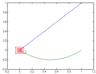
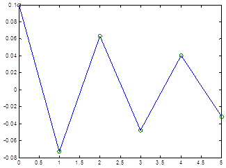
Figure 1. The evolution of citrus starting from P0=1994.
Source: Mulla, 2014 (Ph.D. Thesis)
Case 2
In this case evaluating ![]() instability is noticed in the first years, which is stabilized after three steps.
instability is noticed in the first years, which is stabilized after three steps.
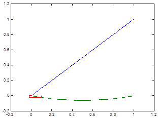
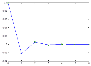
Figure 2. Evolution for citrus starting fromP0=1994 and ![]() .
.
Source: Mulla, 2014 (Ph.D. Thesis)
In case 3 and 4 stability is studied for time intervals ![]() and
and![]() starting from year 2006.
starting from year 2006.
Case 3
![]() .
.
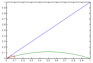
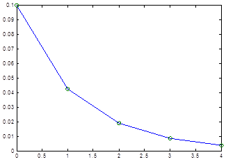
Figure 3. Evolution of citrus starting from P0=2006 and![]() .
.
Source: Mulla, 2014 (Ph.D. Thesis)
Case 4
![]() .
.
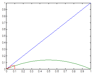
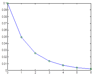
Figure 4. Evolution for citrus starting from P0=2006 and ![]() .
.
Source: Mulla, 2014 (Ph.D. Thesis)
For the culture of wheat utilizing data from year 2004-2012 and using equal time intervals, correspondingly![]() , coefficients of growth and maximal values are obtained as in the table below:
, coefficients of growth and maximal values are obtained as in the table below:
Table 3. Coefficients r and M for different time intervals.
| t1 | 2 | 3 | 4 |
| r | -0.1392 | -0.1322 | 0.3541 |
| M | 248.9395 | 283.537 | 10317 |
Source: Mulla, 2014(Ph.D. Thesis)
Case 5
The following graph shows Cobweb model for results from years 2004-2008, using time intervals ![]() , growth coefficient is
, growth coefficient is ![]() , starting from
, starting from![]() .
.
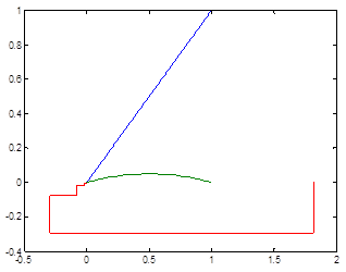
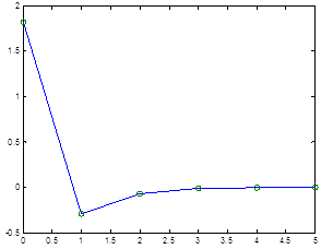
Figure 5. Evolution for wheat starting from P0=2004 and ![]() .
.
Source: Mulla, 2014 (Ph.D. Thesis)
Case 6
This is an application of Cobweb model with results from years 2004-2010, using time intervals![]() , growth coefficient is
, growth coefficient is![]() , starting from
, starting from![]() . The graph reveals that during the first years of the studied interval there is no stability, after 2008 the model is stable.
. The graph reveals that during the first years of the studied interval there is no stability, after 2008 the model is stable.
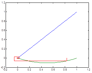
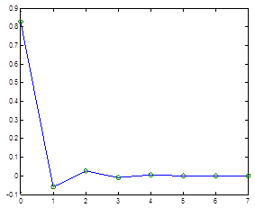
Figure 6. Evolution for wheat starting from P0=2004 and ![]() .
.
Source: Mulla, 2014 (Ph.D. Thesis)
Case 7
This is an application of Cobweb model with results from years 2004-2012, using time intervals ![]() , growth coefficient is
, growth coefficient is ![]() , starting from
, starting from ![]() . In this case, a wider time interval is studied and it is noticed that the stable state is reached in the first two iterations.
. In this case, a wider time interval is studied and it is noticed that the stable state is reached in the first two iterations.
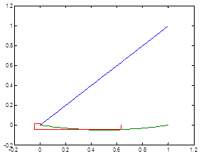
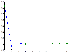
Figure 7. Evolution for wheat starting from P0=2004 and ![]() .
.
Source: Mulla, 2014 (Ph.D. Thesis)
In the two graphs below, we are starting from year 2004 for two different time intervals, ![]() and
and![]() , hence we will have different growth coefficients as exhibited in Table 3, but in this case we have also added predictability, so we have forecasted what evolution this product will follow for year 2016. If we want longer-term predictability, we just have to add time interval in our algorithm, and the advantage if this method compared to other predicting techniques is that the method primarily studies stability and if this is guaranteed then the obtained results will be more reliable.
, hence we will have different growth coefficients as exhibited in Table 3, but in this case we have also added predictability, so we have forecasted what evolution this product will follow for year 2016. If we want longer-term predictability, we just have to add time interval in our algorithm, and the advantage if this method compared to other predicting techniques is that the method primarily studies stability and if this is guaranteed then the obtained results will be more reliable.
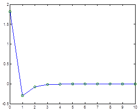
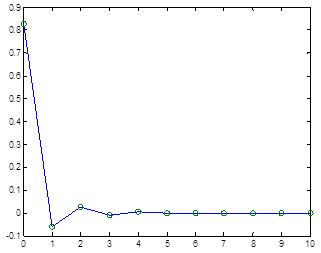
Figure 8. Evolution for wheat for time interval 2004-2014 (P0=2004), for ![]() ,
, ![]() .
.
Source: Mulla, 2014 (Ph.D. Thesis)
As revealed by the graph, there is stability for the period before predicting and this makes prediction difficult. The exact values (first row) and the predicted one (row 2) of wheat price which are connected with graphical representations above are given in the table below.
Table 4. Price of wheat in years and the predicted values.
| Year | 2004 | 2005 | 2006 | 2007 | 2008 | 2009 | 2010 | 2011 | 2012 | 2013 | 2014 | 2015 | 2016 |
| Price | 32 | 31 | 27 | 31 | 45 | 37 | 39 | 36 | - | - | - | - | - |
| Price(p) | 32 | 33.9 | 29.8 | 35 | 35.1 | 37.08 | 37.56 | 32.01 | 32.5 | 32.95 | 33.02 | 33.1 | 33.23 |
Source: Mulla, 2014(Ph.D. Thesis)
Studying closely all the products it is noticed that the best stability if for wheat, and this is justified by the fact that this is a product which in our country has not been imported very often and the interventions with different policies, like decrease or instant removals of import taxes have not been apparent.
For instance, in the case of citrus, import duties have been drastically remove and this has led to instability for the market of this product.
Predictions are necessary to plan, to form decisions, to understand and implement prospective solutions.
6. Conclusions
Starting from the limitations of using linear models, the importance and efficacy of using nonlinear models is highlighted, whose stability is tested with actual data. The test conducted with agricultural data for some of the agricultural products reveals the discrete logistic model is a cobweb model, through which we can make prediction for future years. Evidence from(Boussard and Gérard, 1994) show the positive relationship between price stability and production increase.
During transition years it can not be talked about a planned, stable and well-directed development of agriculture. The application of the exhibited model is a very good way to orient production and market towards stable equilibrium, since during recent years the structures and characteristics of agricultural economy have evolved in a complex and undefined way.
Price tendencies in the market should be analyzed so that rational decision-making on production is taken. Different natural factors in agriculture, absence of infrastructure and marketing, supermarket networks, allocation logistics, securing efficient transportation, stocking, trade etc., dictate fluctuations in production cycle, but determining the tendency to go towards equilibrium point remains the most important thing. Another important challenge is transforming agriculture in a modern sector of market economy, by formulating supportive and integrating economic policies to make Albanian agricultural products competitive in the European Union market.
References
- Anokye M., Oduro F., (2013). Cobweb with buffer stock for the stabilization of tomato prices in Ghana, Journal of Management nad Sustainability. 3 (1). pp. 155-165.
- FinkenstädtB., and Kuhbier P., (1992). Chaotic dynamics in agricultural markets. Springer. 37(1)pp 73-96.
- Bohner M., Warth H., (2008). Logistic dynamic equations in population models. Missouri University of Science and Technology. http://atlasconferences.com/c/ a/w/w/46.htm [Accessed January, 2013].
- Boussard, J.M., and Gérard, F., (1994). Stabilisation des prix et offreagricole in: M. Benoit-cattin, M. Griffon and P. Guillaumonteds (eds), Economics ofagricultural policies in developing countries. Paris: RFSP. Pp. 319-335.
- Zhang, Q., Liu, J. and Luo, ZH, (2015)Dynamical behavior of a third-order rational fuzzy difference equation Advances in Difference Equations. 108(1). pp. 1-18.
- Finkenstadt, B., (1995), Nonlinear Dynamics in Economics: A theoretical and Statistical Approach to Agricultural Markets: Lecture Notes in Economics and Mathematical System. Journal of Economic Literature. 34(4).
- Gonze, G., (2013) The logistic equation, Belgium, pp.1-22.
- Hommes, C. H., (1994),Dynamics of the cobweb model with adaptive expectations and nonlinear supply and demand, Journal of Economic Behaviour & Organization, 24(3) pp.315-335.
- Hommes, C., (2013), Behavioral Rationality and Heterogeneous Expectations in Complex Economic Systems. Cambridge: Cambridge University Press.
- Neusser, K., (2008). Difference Equations for Economists:http://www.vul.unibe.ch/studies/3107_e/DifferenceEquations.pdfMatsumoto A. (1999). Preferable disequilibrum in a nonlinear cobweb economy. Annals of Operations Research, 89. pp.101-123.
- Mulla,P., (2012). Modelimimatematik i disaproblemevedhestabiliteti i tyre:Modeli Cobweb. Albanian Socio Economic Review. 2(71). pp.75-82.
- Mulla, P.,Xhaja,E.,Hoxha, F., (2014). The numerical simulation of nonlinear cobweb model in MATLAB. The Albanian Journal of Natural and Technical Sciences. 36(1).
- Mulla, P., Vegetable price fluctuation in Albania: A nonlinear model for its study. Mediterranean Journal of Social Sciences. 5(2). Pp. 477-482.
- Mulla, P. 2014. The stability of solutions of difference equations and applications in economics. PhD. Thesis. Faculty of natural Sciences, Albania.
- Drejtoria e Bujqësisë e RrethitSarandëdheMinistria e Bujqësisë,UshqimitdheMbrojtjessëKonsumatorit: Vjetaristatistikor. Instituti i Statistikave:www.instat.gov.al [Accessed December, 2014].
- Republika e shqipërisë, Instituti i statistikave. 2013www.instat.gov.al. [Accessed November, 2014].
- Ramos, R. A. (2013). Logistic function as a forecasting model: It’s application to business and economics, International Journal of Engineering and Applied Sciences.2(3). Pp. 29-36.
- Agarwal,P.R., El-Sayed,AMA., and Salman SM., (2013). Fractional-order Chua’s system: discretization,bifurcation and chaos. Advances in Difference Equations.320(1). pp.1-13.


