
American Journal of Economics, Finance and Management, Vol. 1, No. 5, October 2015 Publish Date: Jun. 16, 2015 Pages: 346-361
The Analysis of the Influence of Debt Financing on the Efficiency of Investment Projects in the Perpetuity (Modigliani–Miller) Approximation
P. N. Brusov1, *, T. V. Filatova2, N. P. Orekhova3, 5, I. K. Shevchenko4, A. Y. Arkhipov5, V. L. Kulik6
1Applied Mathematics Department, Financial University under the Government of Russian Federation, Moscow, Russia
2Dean of GMM Faculty, Financial University under the Government of Russian Federation, Moscow, Russia
3Investment and Taxation Laboratory, Research Consortium of Universities of the South of Russia, Rostov-on-Don, Russia
4Research and Innovation Projects, Southern Federal University, Rostov-on-Don, Russia
5High School of Business, Southern Federal University, Rostov-on-Don, Russia
6Management Department, Financial University under the Government of Russian Federation, Moscow, Russia
Abstract
The analysis of effectiveness of investment projects within the perpetuity (Modigliani–Miller) approximation (Modigliani et al 1958, 1963, 1966) has been done. Based on the obtained in previous papers results for NPV (Brusov et al 2011a, b, c, d, e; 2012 a, b; 2013 a, b, c; 2014 a, b; Filatova et al 2008) we analyze the effectiveness of investment projects for three cases.
Keywords
Received: April 8, 2015
Accepted: April 26, 2015
Published online: June 14, 2015
@ 2015 The Authors. Published by American Institute of Science. This Open Access article is under the CC BY-NC license. http://creativecommons.org/licenses/by-nc/4.0/
Contents
1. Introduction 2. The Effectiveness of the Investment Project from the Perspective of the Equity Holders Only 2.1. With the Division of Credit and Investment Flows 2.2. Without Flows Separation 3. The Effectiveness of the Investment Project from the Perspective of the Equity and Debt Owners 3.1. With the Division of Credit and Investment Flows 3.2. Without Flows Separation 4. Conclusions
1. Introduction
In this paper we conduct the analysis of effectiveness of investment projects within the perpetuity (Modigliani–Miller) approximation (Modigliani et al 1958, 1963, 1966). Based on the obtained in previous papers results for NPV (Brusov P, Filatova T, Orehova N, Eskindarov M 2015, Brusov et al 2011a,b,c,d,e; 2012 a, b; 2013 a, b, c; 2014 a, b; Filatova et al 2008) we analyze the effectiveness of investment projects for three cases:
1) at a constant difference between equity cost (at ![]() ) and debt cost
) and debt cost ![]() ;
;
2) at a constant equity cost (at ![]() ) and varying debt cost
) and varying debt cost ![]() ;
;
3) at a constant debt cost ![]() and varying equity cost (at
and varying equity cost (at ![]() )
) ![]() .
.
The dependence of NPV on investment value and/or equity value will be also analyzed. The results are shown in the form of tables and graphs.
It should be noted that the obtained tables have played an important practical role in determining of the optimal, or acceptable debt level, at which the project remains effective. The optimal debt level there is for the situation, when in the dependence of NPV on leverage level L there is an optimum (leverage level value, at which NPV reaches a maximum value. An acceptable debt level there is for the situation, when NPV decreases with leverage. And, finally, it is possible that NPV is growing with leverage. In this case, an increase in borrowing leads to increased effectiveness of investment projects, and their limit is determined by financial sustainability of investing company.
2. The Effectiveness of the Investment Project from the Perspective of the Equity Holders Only
2.1. With the Division of Credit and Investment Flows
At a constant value of the total invested capital (I = const)
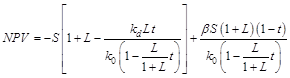
![]() (1)
(1)
1) At the constant values of ![]() NPV practically always decreases with leverage. At small L for many pairs of values
NPV practically always decreases with leverage. At small L for many pairs of values ![]() and
and ![]() (for example,
(for example, ![]() (14%) and
(14%) and ![]() (12%) ;
(12%) ; ![]() (18%) and
(18%) and ![]() (16%) and many others) there is an optimum in the dependence of NPV(L) at small
(16%) and many others) there is an optimum in the dependence of NPV(L) at small ![]()
For higher values of ![]() (and, accordingly,
(and, accordingly, ![]() ) curves NPV(L) lie below. With increase of NOI all curves NPV(L) is shifted in parallel upwards.
) curves NPV(L) lie below. With increase of NOI all curves NPV(L) is shifted in parallel upwards.
2) At the constant values of ![]() NPV practically always decreases with leverage, passing through (most often), or not passing (more rarely) through optimum in the dependence of NPV(L) at small
NPV practically always decreases with leverage, passing through (most often), or not passing (more rarely) through optimum in the dependence of NPV(L) at small ![]()
All curves NPV(L) at the constant values of ![]() are started (at L=0) from a single point, and with the increasing of
are started (at L=0) from a single point, and with the increasing of ![]() (and, respectively, a decrease of
(and, respectively, a decrease of ![]() ) curves NPV(L) lie above. With increase of NOI all curve NPV(L) are shifted in parallel upwards practically.
) curves NPV(L) lie above. With increase of NOI all curve NPV(L) are shifted in parallel upwards practically.
3) At the constant values of ![]() NPV practically always decreases with leverage, optimum in the dependence of NPV(L) отсутствует.
NPV practically always decreases with leverage, optimum in the dependence of NPV(L) отсутствует.
All curves NPV(L) at the constant values of ![]() are started (at L=0) from a single point. With the increasing of
are started (at L=0) from a single point. With the increasing of ![]() (and, respectively, a increase of
(and, respectively, a increase of ![]() ) curves NPV(L) is shifted into region of higher NPV values. With increase of NOI all curves NPV(L) are shifted in parallel upwards practically.
) curves NPV(L) is shifted into region of higher NPV values. With increase of NOI all curves NPV(L) are shifted in parallel upwards practically.
Table 1. Dependence of NPV on leverage level NOI=1200 I=2000, k0-kd=const.
| k0 | kd\L | 0.0 | 0.5 | 1.0 | 1.5 | 2.0 | 2.5 | 3.0 | 3.5 | 4.0 | 4.5 | |
| 1 | 0.08 | 0.06 | 10000.0 | 9042.4 | 8200.0 | 7470.8 | 6838.1 | 6285.7 | 5800.0 | 5369.9 | 4986.7 | 4643.1 |
| 2 | 0.10 | 0.08 | 7600.0 | 7022.2 | 6475.9 | 5981.9 | 5539.4 | 5142.9 | 4786.5 | 4465.0 | 4173.7 | 3908.7 |
| 3 | 0.14 | 0.12 | 4857.1 | 4619.8 | 4353.8 | 4093.7 | 3848.1 | 3619.0 | 3406.4 | 3209.1 | 3025.9 | 2855.6 |
| 4 | 0.18 | 0.16 | 3333.3 | 3239.7 | 3098.0 | 2945.9 | 2795.0 | 2649.4 | 2510.5 | 2378.9 | 2254.4 | 2136.8 |
| 5 | 0.24 | 0.22 | 2000.0 | 2004.3 | 1950.0 | 1876.4 | 1796.1 | 1714.3 | 1633.3 | 1554.4 | 1477.9 | 1404.2 |
| 6 | 0.30 | 0.28 | 1200.0 | 1250.2 | 1238.0 | 1203.0 | 1158.2 | 1109.2 | 1058.6 | 1007.7 | 957.4 | 907.9 |
| 7 | 0.36 | 0.34 | 666.7 | 742.0 | 753.2 | 740.0 | 715.6 | 685.7 | 652.9 | 618.8 | 584.2 | 549.5 |
| 8 | 0.40 | 0.38 | 400.0 | 486.3 | 507.7 | 504.2 | 488.9 | 467.5 | 442.9 | 416.4 | 389.0 | 361.2 |
| 9 | 0.44 | 0.42 | 181.8 | 276.2 | 305.3 | 309.0 | 300.6 | 285.7 | 267.2 | 246.6 | 224.8 | 202.3 |
| 10 | 0.10 | 0.06 | 7600.0 | 6409.2 | 5472.7 | 4726.5 | 4120.3 | 3619.0 | 3198.0 | 2839.4 | 2530.5 | 2261.7 |
| 11 | 0.12 | 0.08 | 6000.0 | 5192.2 | 4515.8 | 3954.3 | 3484.1 | 3085.7 | 2744.4 | 2449.0 | 2191.0 | 1963.6 |
| 12 | 0.16 | 0.12 | 4000.0 | 3587.9 | 3200.0 | 2855.4 | 2552.4 | 2285.7 | 2050.0 | 1840.5 | 1653.3 | 1485.2 |
| 13 | 0.20 | 0.16 | 2800.0 | 2577.8 | 2337.9 | 2111.0 | 1903.0 | 1714.3 | 1543.2 | 1388.0 | 1246.8 | 1118.0 |
| 14 | 0.24 | 0.20 | 2000.0 | 1883.3 | 1729.4 | 1573.3 | 1424.6 | 1285.7 | 1157.1 | 1038.4 | 928.7 | 827.3 |
| 15 | 0.30 | 0.26 | 1200.0 | 1171.3 | 1091.6 | 998.6 | 904.0 | 812.0 | 724.2 | 641.2 | 563.0 | 489.4 |
| 16 | 0.36 | 0.32 | 666.7 | 686.5 | 649.0 | 592.9 | 530.8 | 467.5 | 405.3 | 345.0 | 287.2 | 232.0 |
| 17 | 0.40 | 0.36 | 400.0 | 441.0 | 422.2 | 382.9 | 335.6 | 285.7 | 235.5 | 186.1 | 138.2 | 92.0 |
| 18 | 0.44 | 0.40 | 181.8 | 238.6 | 233.9 | 207.2 | 171.4 | 131.9 | 91.0 | 50.2 | 10.1 | -28.9 |
Table 1. (continue)
| k0 | kd\L | 5.0 | 5.5 | 6.0 | 6.5 | 7.0 | 7.5 | 8.0 | 8.5 | 9.0 | 9.5 | 10.0 | |
| 1 | 0.08 | 0.06 | 4333.3 | 4052.7 | 3797.4 | 3564.1 | 3350.0 | 3152.9 | 2970.9 | 2802.3 | 2645.7 | 2499.8 | 2363.6 |
| 2 | 0.10 | 0.08 | 3666.7 | 3444.8 | 3240.8 | 3052.5 | 2878.3 | 2716.6 | 2566.1 | 2425.7 | 2294.4 | 2171.4 | 2055.9 |
| 3 | 0.14 | 0.12 | 2697.0 | 2549.0 | 2410.7 | 2281.1 | 2159.5 | 2045.2 | 1937.6 | 1836.2 | 1740.3 | 1649.6 | 1563.6 |
| 4 | 0.18 | 0.16 | 2025.6 | 1920.6 | 1821.1 | 1726.9 | 1637.7 | 1552.9 | 1472.4 | 1395.9 | 1323.0 | 1253.5 | 1187.2 |
| 5 | 0.24 | 0.22 | 1333.3 | 1265.3 | 1200.0 | 1137.4 | 1077.3 | 1019.6 | 964.3 | 911.1 | 860.0 | 810.9 | 763.6 |
| 6 | 0.30 | 0.28 | 859.6 | 812.7 | 767.1 | 722.9 | 680.1 | 638.7 | 598.5 | 559.7 | 522.2 | 485.8 | 450.6 |
| 7 | 0.36 | 0.34 | 515.2 | 481.3 | 448.1 | 415.6 | 383.9 | 352.9 | 322.8 | 293.4 | 264.8 | 236.9 | 209.8 |
| 8 | 0.40 | 0.38 | 333.3 | 305.7 | 278.3 | 251.4 | 225.0 | 199.1 | 173.7 | 148.9 | 124.7 | 101.0 | 77.9 |
| 9 | 0.44 | 0.42 | 179.5 | 156.6 | 133.9 | 111.4 | 89.1 | 67.2 | 45.7 | 24.6 | 3.8 | -16.5 | -36.4 |
| 10 | 0.10 | 0.06 | 2025.6 | 1816.7 | 1630.5 | 1463.5 | 1313.0 | 1176.5 | 1052.2 | 938.5 | 834.2 | 738.1 | 649.4 |
| 11 | 0.12 | 0.08 | 1761.9 | 1581.7 | 1419.8 | 1273.5 | 1140.7 | 1019.6 | 908.7 | 806.9 | 712.9 | 626.1 | 545.5 |
| 12 | 0.16 | 0.12 | 1333.3 | 1195.6 | 1070.1 | 955.4 | 850.0 | 752.9 | 663.2 | 580.1 | 502.9 | 430.9 | 363.6 |
| 13 | 0.20 | 0.16 | 1000.0 | 891.7 | 791.8 | 699.6 | 614.2 | 534.8 | 460.8 | 391.8 | 327.2 | 266.7 | 209.8 |
| 14 | 0.24 | 0.20 | 733.3 | 646.2 | 565.1 | 489.5 | 419.0 | 352.9 | 291.0 | 232.9 | 178.2 | 126.6 | 77.9 |
| 15 | 0.30 | 0.26 | 420.3 | 355.3 | 294.1 | 236.4 | 182.1 | 130.7 | 82.2 | 36.2 | -7.3 | -48.7 | -88.0 |
| 16 | 0.36 | 0.32 | 179.5 | 129.5 | 82.0 | 36.8 | -6.2 | -47.1 | -86.0 | -123.1 | -158.5 | -192.3 | -224.6 |
| 17 | 0.40 | 0.36 | 47.6 | 5.1 | -35.5 | -74.4 | -111.5 | -147.1 | -181.0 | -213.5 | -244.7 | -274.5 | -303.0 |
| 18 | 0.44 | 0.40 | -66.7 | -103.1 | -138.2 | -171.9 | -204.2 | -235.3 | -265.1 | -293.8 | -321.3 | -347.8 | -373.2 |
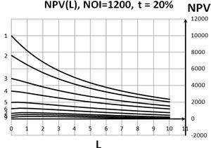
Fig. 1. Dependence of NPV on leverage level at fixed values of ![]() and
and ![]() .
.
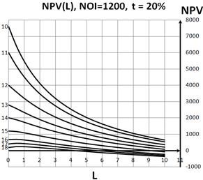
Fig. 2. Dependence of NPV on leverage level at fixed values of ![]() and
and ![]() .
.
At a constant equity value (S = const)
![]() (2)
(2)
1) At the constant values of ![]() NPV practically always decreases with leverage. The optimum in the dependence of NPV(L) has been found for one pair of
NPV practically always decreases with leverage. The optimum in the dependence of NPV(L) has been found for one pair of ![]() and
and ![]() (
(![]() (8%) and
(8%) and ![]() (6%)) only.
(6%)) only.
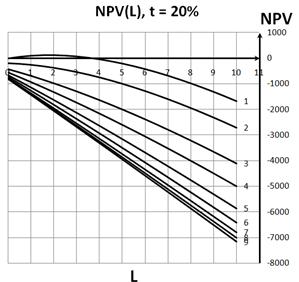
Fig. 3. Dependence of NPV on leverage level at fixed values of ![]() and
and ![]() .
.
All curves NPV(L) at the constant values of ![]() are started (at L=0) from one point and with growth of
are started (at L=0) from one point and with growth of ![]() (and, accordingly,
(and, accordingly, ![]() ) all curves NPV(L) lie below. With growth of
) all curves NPV(L) lie below. With growth of ![]() density of curves NPV(L) increases.
density of curves NPV(L) increases.
2) At the constant values of ![]() NPV practically always decreases with leverage. Optimum in the dependence of NPV(L) is absent.
NPV practically always decreases with leverage. Optimum in the dependence of NPV(L) is absent.
All curves NPV(L) at the constant values of ![]() are started (at L=0) from one point and with growth of
are started (at L=0) from one point and with growth of ![]() (and, respectively, a decrease of
(and, respectively, a decrease of ![]() ) all curves NPV (L) are shifted upwards. With growth of
) all curves NPV (L) are shifted upwards. With growth of ![]() density of curves NPV(L) increases.
density of curves NPV(L) increases.
3) At the constant values of ![]() NPV practically always decreases with leverage. The optimum in the dependence of NPV(L) has been found for one pair of
NPV practically always decreases with leverage. The optimum in the dependence of NPV(L) has been found for one pair of ![]() and
and ![]() (
(![]() (8%) and
(8%) and ![]() (6%)) only.
(6%)) only.
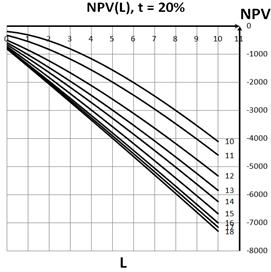
Fig. 4. Dependence of NPV on leverage level at fixed values of ![]() and
and ![]() .
.
All curves NPV(L) at the constant values of ![]() are started (at L=0) from one point and with growth of
are started (at L=0) from one point and with growth of ![]() (and, respectively, an increase of
(and, respectively, an increase of ![]() ) curves NPV (L) are shifted into region of smaller NPV values. With growth of
) curves NPV (L) are shifted into region of smaller NPV values. With growth of ![]() density of curves NPV(L) increases.
density of curves NPV(L) increases.
1) At the constant values of ![]() NPV practically always decreases with leverage. The optimum in the dependence of NPV(L) has been found for one pair of
NPV practically always decreases with leverage. The optimum in the dependence of NPV(L) has been found for one pair of ![]() and
and ![]() (
(![]() (8%) and
(8%) and ![]() (6%)) only. All curves NPV(L) at the constant values of
(6%)) only. All curves NPV(L) at the constant values of ![]() are started (at L=0) from one point and with growth of
are started (at L=0) from one point and with growth of ![]() (and, respectively,
(and, respectively, ![]() ) curves NPV (L) lie below.
) curves NPV (L) lie below.
With growth of ![]() density of curves NPV(L) increases.
density of curves NPV(L) increases.
2) At the constant values of ![]() NPV practically always decreases with leverage. Optimum in the dependence of NPV(L) is absent.
NPV practically always decreases with leverage. Optimum in the dependence of NPV(L) is absent.
All curves NPV(L) at the constant values of ![]() are started (at L=0) from one point and with growth of
are started (at L=0) from one point and with growth of ![]() (and, respectively, a decrease of
(and, respectively, a decrease of ![]() ) curves NPV (L) are shifted upwards. With growth of
) curves NPV (L) are shifted upwards. With growth of ![]() density of curves NPV(L) increases.
density of curves NPV(L) increases.
3) At the constant values of ![]() NPV practically always decreases with leverage. The optimum in the dependence of NPV(L) has been found for one pair of
NPV practically always decreases with leverage. The optimum in the dependence of NPV(L) has been found for one pair of ![]() and
and ![]() (
(![]() (8%) and
(8%) and ![]() (6%)) only. All curves NPV(L) at the constant values of
(6%)) only. All curves NPV(L) at the constant values of ![]() are started (at L=0) from one point and with growth of
are started (at L=0) from one point and with growth of ![]() (and, respectively, an increase of
(and, respectively, an increase of ![]() ) curves NPV (L) are shifted into region of smaller NPV values. With growth of
) curves NPV (L) are shifted into region of smaller NPV values. With growth of ![]() density of curves NPV(L) increases.
density of curves NPV(L) increases.
Table 2. Dependence of NPV on leverage level S=1000 b=0.1, k0-kd=const.
| k0 | kd\L | 0.0 | 0.5 | 1.0 | 1.5 | 2.0 | 2.5 | 3.0 | 3.5 | 4.0 | 4.5 | |
| 1 | 0.08 | 0.06 | 0.0 | 63.4 | 104.8 | 125.6 | 127.3 | 111.1 | 78.3 | 29.8 | -33.3 | -110.2 |
| 2 | 0.10 | 0.08 | -200.0 | -223.5 | -261.5 | -313.2 | -377.8 | -454.5 | -542.9 | -642.1 | -751.7 | -871.2 |
| 3 | 0.14 | 0.12 | -428.6 | -554.9 | -688.9 | -830.1 | -978.4 | -1133.3 | -1294.7 | -1462.3 | -1635.9 | -1815.2 |
| 4 | 0.18 | 0.16 | -555.6 | -740.7 | -930.4 | -1124.7 | -1323.4 | -1526.3 | -1733.3 | -1944.3 | -2159.2 | -2377.8 |
| 5 | 0.24 | 0.22 | -666.7 | -904.1 | -1144.3 | -1387.0 | -1632.3 | -1880.0 | -2130.2 | -2382.7 | -2637.5 | -2894.6 |
| 6 | 0.30 | 0.28 | -733.3 | -1002.6 | -1273.7 | -1546.4 | -1820.8 | -2096.8 | -2374.4 | -2653.5 | -2934.2 | -3216.4 |
| 7 | 0.36 | 0.34 | -777.8 | -1068.5 | -1360.4 | -1653.6 | -1947.8 | -2243.2 | -2539.8 | -2837.4 | -3136.2 | -3436.0 |
| 8 | 0.40 | 0.38 | -800.0 | -1101.5 | -1404.0 | -1707.4 | -2011.8 | -2317.1 | -2623.3 | -2930.4 | -3238.5 | -3547.4 |
| 9 | 0.44 | 0.42 | -818.2 | -1128.5 | -1439.6 | -1751.6 | -2064.3 | -2377.8 | -2692.0 | -3007.0 | -3322.8 | -3639.3 |
| 10 | 0.10 | 0.06 | -200.0 | -246.2 | -318.5 | -414.3 | -531.0 | -666.7 | -819.4 | -987.5 | -1169.7 | -1364.7 |
| 11 | 0.12 | 0.08 | -333.3 | -432.3 | -550.0 | -684.8 | -835.3 | -1000.0 | -1177.8 | -1367.6 | -1568.4 | -1779.5 |
| 12 | 0.16 | 0.12 | -500.0 | -668.3 | -847.6 | -1037.2 | -1236.4 | -1444.4 | -1660.9 | -1885.1 | -2116.7 | -2355.1 |
| 13 | 0.20 | 0.16 | -600.0 | -811.8 | -1030.8 | -1256.6 | -1488.9 | -1727.3 | -1971.4 | -2221.1 | -2475.9 | -2735.6 |
| 14 | 0.24 | 0.20 | -666.7 | -908.2 | -1154.8 | -1406.3 | -1662.5 | -1923.1 | -2187.9 | -2456.7 | -2729.4 | -3005.8 |
| 15 | 0.30 | 0.26 | -733.3 | -1005.3 | -1280.5 | -1559.0 | -1840.5 | -2125.0 | -24 3 | -2702.4 | -2995.2 | -3290.5 |
| 16 | 0.36 | 0.32 | -777.8 | -1070.3 | -1365.2 | -1662.4 | -1961.7 | -2263.2 | -2566.7 | -2872.2 | -3179.6 | -3488.9 |
| 17 | 0.40 | 0.36 | -800.0 | -1103.0 | -1407.8 | -1714.6 | -2023.1 | -2333.3 | -2645.3 | -2958.9 | -3274.1 | -3590.8 |
| 18 | 0.44 | 0.40 | -818.2 | -1129.7 | -1442.9 | -1757.5 | -2073.7 | -2391.3 | -2710.3 | -3030.8 | -3352.5 | -3675.6 |
Table 2. (Continue)
| k0 | kd\L | 5.0 | 5.5 | 6.0 | 6.5 | 7.0 | 7.5 | 8.0 | 8.5 | 9.0 | 9.5 | 10.0 | |
| 1 | 0.08 | 0.06 | -200.0 | -302.0 | -415.4 | -539.6 | -674.1 | -818.2 | -971.4 | -1133.3 | -1303.4 | -1481.4 | -1666.7 |
| 2 | 0.10 | 0.08 | -1000.0 | -1137.7 | -1283.9 | -1438.1 | -1600.0 | -1769.2 | -1945.5 | -2128.4 | -2317.6 | -2513.0 | -2714.3 |
| 3 | 0.14 | 0.12 | -2000.0 | -2190.1 | -2385.4 | -2585.5 | -2790.5 | -3000.0 | -3214.0 | -3432.2 | -3654.5 | -3880.9 | -4111.1 |
| 4 | 0.18 | 0.16 | -2600.0 | -2825.7 | -3054.9 | -3287.4 | -3523.1 | -3761.9 | -4003.8 | -4248.6 | -4496.3 | -4746.8 | -5000.0 |
| 5 | 0.24 | 0.22 | -3153.8 | -3415.3 | -3678.8 | -3944.4 | -4211.9 | -4481.5 | -4752.9 | -5026.3 | -5301.4 | -5578.4 | -5857.1 |
| 6 | 0.30 | 0.28 | -3500.0 | -3785.1 | -4071.6 | -4359.5 | -4648.8 | -4939.4 | -5231.3 | -5524.6 | -5819.0 | -6114.8 | -6411.8 |
| 7 | 0.36 | 0.34 | -3736.8 | -4038.7 | -4341.7 | -4645.6 | -4950.5 | -5256.4 | -5563.3 | -5871.1 | -6179.8 | -6489.4 | -6800.0 |
| 8 | 0.40 | 0.38 | -3857.1 | -4167.8 | -4479.2 | -4791.5 | -5104.7 | -5418.6 | -5733.3 | -6048.8 | -6365.1 | -6682.2 | -7000.0 |
| 9 | 0.44 | 0.42 | -3956.5 | -4274.5 | -4593.1 | -49 4 | -5232.5 | -5553.2 | -5874.6 | -6196.6 | -6519.3 | -6842.7 | -7166.7 |
| 10 | 0.10 | 0.06 | -1571.4 | -1788.9 | -2016.2 | -2252.6 | -2497.4 | -2750.0 | -3009.8 | -3276.2 | -3548.8 | -3827.3 | -4111.1 |
| 11 | 0.12 | 0.08 | -2000.0 | -2229.3 | -2466.7 | -2711.6 | -2963.6 | -3222.2 | -3487.0 | -3757.4 | -4033.3 | -4314.3 | -4600.0 |
| 12 | 0.16 | 0.12 | -2600.0 | -2851.0 | -3107.7 | -3369.8 | -3637.0 | -3909.1 | -4185.7 | -4466.7 | -4751.7 | -5040.7 | -5333.3 |
| 13 | 0.20 | 0.16 | -3000.0 | -3268.9 | -3541.9 | -3819.0 | -4100.0 | -4384.6 | -4672.7 | -4964.2 | -5258.8 | -5556.5 | -5857.1 |
| 14 | 0.24 | 0.20 | -3285.7 | -3569.0 | -3855.6 | -4145.2 | -4437.8 | -4733.3 | -5031.6 | -5332.5 | -5635.9 | -5941.8 | -6250.0 |
| 15 | 0.30 | 0.26 | -3588.2 | -3888.4 | -4190.8 | -4495.5 | -4802.2 | -5111.1 | -5422.0 | -5734.8 | -6049.5 | -6366.0 | -6684.2 |
| 16 | 0.36 | 0.32 | -3800.0 | -41 9 | -4427.5 | -4743.7 | -5061.5 | -5381.0 | -5701.9 | -6024.3 | -6348.1 | -6673.4 | -7000.0 |
| 17 | 0.40 | 0.36 | -3909.1 | -4228.8 | -4550.0 | -4872.6 | -5196.5 | -5521.7 | -5848.3 | -6176.1 | -6505.1 | -6835.3 | -7166.7 |
| 18 | 0.44 | 0.40 | -4000.0 | -4325.6 | -4652.5 | -4980.5 | -5309.7 | -5640.0 | -5971.4 | -6303.9 | -6637.5 | -6972.1 | -7307.7 |
2.2. Without Flows Separation
At a constant investment value (I = const)
![]() (3)
(3)
At the constant values of ![]() NPV demonstrates a limited growth with leverage with output into saturation regime. The main increase in NPV occurs when
NPV demonstrates a limited growth with leverage with output into saturation regime. The main increase in NPV occurs when ![]() . With growth of
. With growth of ![]() (and
(and ![]() ) the сurves NPV(L) are lowered. Optimum in the dependence of NPV(L) is absent.
) the сurves NPV(L) are lowered. Optimum in the dependence of NPV(L) is absent.
With growth of NOI all curves NPV(L) are shifted practically parallel upwards.
2) At the constant values of ![]() NPV demonstrates a limited growth with leverage with output into saturation regime. All curves NPV(L) at the constant values of
NPV demonstrates a limited growth with leverage with output into saturation regime. All curves NPV(L) at the constant values of![]() and different values of
and different values of ![]() are started (at L=0) from one point, the higher values of
are started (at L=0) from one point, the higher values of ![]() correspond to more low lying curves NPV(L). Optimum in dependence of NPV(L) is absent. With growth of NOI all curves NPV(L) are shifted practically parallel upwards.
correspond to more low lying curves NPV(L). Optimum in dependence of NPV(L) is absent. With growth of NOI all curves NPV(L) are shifted practically parallel upwards.
3) At the constant values of ![]() NPV grows with leverage with output into saturation regime. All curves NPV(L) at the constant values of
NPV grows with leverage with output into saturation regime. All curves NPV(L) at the constant values of ![]() and different values of
and different values of ![]() are started (at L=0) from one point, the higher values of
are started (at L=0) from one point, the higher values of ![]() (and higher values of
(and higher values of ![]() ) correspond to more low lying curves NPV(L). Optimum in dependence of NPV(L) is absent.
) correspond to more low lying curves NPV(L). Optimum in dependence of NPV(L) is absent.
Table 3. Dependence of NPV on leverage level NOI=1200 I=2000, k0-kd=const.
| k0 | kd\L | 0.0 | 0.5 | 1.0 | 1.5 | 2.0 | 2.5 | 3.0 | 3.5 | 4.0 | 4.5 | |
| 1 | 0.08 | 0.06 | 10000.0 | 11095.2 | 11666.7 | 12018.2 | 12256.4 | 12428.6 | 12558.8 | 12660.8 | 12742.9 | 12810.3 |
| 2 | 0.10 | 0.08 | 7600.0 | 8495.2 | 8955.6 | 9236.4 | 9425.6 | 9561.9 | 9664.7 | 9745.0 | 9809.5 | 9862.5 |
| 3 | 0.14 | 0.12 | 4857.1 | 5523.8 | 5857.1 | 6057.1 | 6190.5 | 6285.7 | 6357.1 | 64 7 | 6457.1 | 6493.5 |
| 4 | 0.18 | 0.16 | 3333.3 | 3873.0 | 4135.8 | 4290.9 | 4393.2 | 4465.6 | 4519.6 | 4561.4 | 4594.7 | 4621.9 |
| 5 | 0.24 | 0.22 | 2000.0 | 2428.6 | 2629.6 | 2745.5 | 2820.5 | 2873.0 | 2911.8 | 2941.5 | 2965.1 | 2984.2 |
| 6 | 0.30 | 0.28 | 1200.0 | 1561.9 | 1725.9 | 1818.2 | 1876.9 | 1917.5 | 1947.1 | 1969.6 | 1987.3 | 2001.6 |
| 7 | 0.36 | 0.34 | 666.7 | 984.1 | 1123.5 | 1200.0 | 1247.9 | 1280.4 | 1303.9 | 1321.6 | 1335.4 | 1346.5 |
| 8 | 0.40 | 0.38 | 400.0 | 695.2 | 822.2 | 890.9 | 933.3 | 961.9 | 982.4 | 997.7 | 1009.5 | 1019.0 |
| 9 | 0.44 | 0.42 | 181.8 | 458.9 | 575.8 | 638.0 | 676.0 | 701.3 | 719.3 | 732.6 | 742.9 | 751.0 |
| 10 | 0.10 | 0.06 | 7600.0 | 8609.5 | 9133.3 | 9454.5 | 9671.8 | 9828.6 | 9947.1 | 10039.8 | 10114.3 | 10175.5 |
| 11 | 0.12 | 0.08 | 6000.0 | 6857.1 | 7296.3 | 7563.6 | 7743.6 | 7873.0 | 7970.6 | 8046.8 | 8107.9 | 8158.1 |
| 12 | 0.16 | 0.12 | 4000.0 | 4666.7 | 5000.0 | 5200.0 | 5333.3 | 5428.6 | 5500.0 | 5555.6 | 5600.0 | 5636.4 |
| 13 | 0.20 | 0.16 | 2800.0 | 3352.4 | 3622.2 | 3781.8 | 3887.2 | 3961.9 | 4017.6 | 4060.8 | 4095.2 | 4123.3 |
| 14 | 0.24 | 0.20 | 2000.0 | 2476.2 | 2703.7 | 2836.4 | 2923.1 | 2984.1 | 3029.4 | 3064.3 | 3092.1 | 3114.6 |
| 15 | 0.30 | 0.26 | 1200.0 | 1600.0 | 1785.2 | 1890.9 | 1959.0 | 2006.3 | 2041.2 | 2067.8 | 2088.9 | 2105.9 |
| 16 | 0.36 | 0.32 | 666.7 | 1015.9 | 1172.8 | 1260.6 | 1316.2 | 1354.5 | 1382.4 | 1403.5 | 1420.1 | 1433.5 |
| 17 | 0.40 | 0.36 | 400.0 | 723.8 | 866.7 | 945.5 | 994.9 | 1028.6 | 1052.9 | 1071.3 | 1085.7 | 1097.2 |
| 18 | 0.44 | 0.40 | 181.8 | 484.8 | 616.2 | 687.6 | 731.9 | 761.9 | 783.4 | 799.6 | 8 1 | 822.1 |
Table 3. (continue)
| k0 | kd\L | 5.0 | 5.5 | 6.0 | 6.5 | 7.0 | 7.5 | 8.0 | 8.5 | 9.0 | 9.5 | 10.0 | |
| 1 | 0.08 | 0.06 | 12866.7 | 12914.5 | 12955.7 | 12991.4 | 13022.7 | 13050.4 | 13075.1 | 13097.2 | 13117.1 | 13135.1 | 13151.5 |
| 2 | 0.10 | 0.08 | 9906.7 | 9944.2 | 9976.4 | 10004.3 | 10028.8 | 10050.4 | 10069.7 | 10086.9 | 10102.4 | 10116.5 | 10129.3 |
| 3 | 0.14 | 0.12 | 6523.8 | 6549.5 | 6571.4 | 6590.5 | 6607.1 | 6621.8 | 6634.9 | 6646.6 | 6657.1 | 6666.7 | 6675.3 |
| 4 | 0.18 | 0.16 | 4644.4 | 4663.5 | 4679.8 | 4693.9 | 4706.2 | 4717.1 | 4726.7 | 4735.3 | 4743.1 | 4750.1 | 4756.5 |
| 5 | 0.24 | 0.22 | 3000.0 | 3013.3 | 3024.6 | 3034.4 | 3042.9 | 3050.4 | 3057.1 | 3063.0 | 3068.3 | 3073.1 | 3077.4 |
| 6 | 0.30 | 0.28 | 2013.3 | 2023.2 | 2031.5 | 2038.7 | 2044.9 | 2050.4 | 2055.3 | 2059.6 | 2063.4 | 2066.9 | 2070.0 |
| 7 | 0.36 | 0.34 | 1355.6 | 1363.1 | 1369.5 | 1374.9 | 1379.6 | 1383.8 | 1387.4 | 1390.6 | 1393.5 | 1396.1 | 1398.4 |
| 8 | 0.40 | 0.38 | 1026.7 | 1033.0 | 1038.4 | 1043.0 | 1047.0 | 1050.4 | 1053.5 | 1056.1 | 1058.5 | 1060.7 | 1062.6 |
| 9 | 0.44 | 0.42 | 757.6 | 763.0 | 767.6 | 771.5 | 774.8 | 777.7 | 780.2 | 782.5 | 784.5 | 786.3 | 787.9 |
| 10 | 0.10 | 0.06 | 10226.7 | 10270.1 | 10307.4 | 10339.8 | 10368.2 | 10393.3 | 10415.6 | 10435.6 | 10453.7 | 10470.0 | 10484.8 |
| 11 | 0.12 | 0.08 | 8200.0 | 8235.5 | 8266.0 | 8292.5 | 8315.7 | 8336.1 | 8354.4 | 8370.7 | 8385.4 | 8398.7 | 8410.8 |
| 12 | 0.16 | 0.12 | 5666.7 | 5692.3 | 5714.3 | 5733.3 | 5750.0 | 5764.7 | 5777.8 | 5789.5 | 5800.0 | 5809.5 | 5818.2 |
| 13 | 0.20 | 0.16 | 4146.7 | 4166.4 | 4183.3 | 4197.8 | 4210.6 | 4221.8 | 4231.8 | 4240.8 | 4248.8 | 4256.0 | 4262.6 |
| 14 | 0.24 | 0.20 | 3133.3 | 3149.1 | 3162.6 | 3174.2 | 3184.3 | 3193.3 | 3201.2 | 3208.3 | 3214.6 | 3220.4 | 3225.6 |
| 15 | 0.30 | 0.26 | 2120.0 | 2131.8 | 2141.9 | 2150.5 | 2158.1 | 2164.7 | 2170.6 | 2175.8 | 2180.5 | 2184.7 | 2188.6 |
| 16 | 0.36 | 0.32 | 1444.4 | 1453.6 | 1461.4 | 1468.1 | 1473.9 | 1479.0 | 1483.5 | 1487.5 | 1491.1 | 1494.3 | 1497.2 |
| 17 | 0.40 | 0.36 | 1106.7 | 1114.5 | 1121.2 | 1126.9 | 1131.8 | 1136.1 | 1139.9 | 1143.3 | 1146.3 | 1149.1 | 1151.5 |
| 18 | 0.44 | 0.40 | 830.3 | 837.1 | 842.8 | 847.7 | 851.9 | 855.6 | 858.9 | 861.7 | 864.3 | 866.6 | 868.7 |
At a constant equity value (S = const)
![]() (4)
(4)
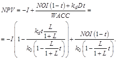
At the constant values of ![]() NPV shows as an unlimited growth with leverage and unlimited descending with leverage. It is interesting to note, that the credit rate value
NPV shows as an unlimited growth with leverage and unlimited descending with leverage. It is interesting to note, that the credit rate value ![]() turns out to be a border at all surveyed values of
turns out to be a border at all surveyed values of ![]() , equal to 2%, 4%, 6%,10% (it separates the growth of NPV with leverage from descending of NPV with leverage). In other words, with growth of
, equal to 2%, 4%, 6%,10% (it separates the growth of NPV with leverage from descending of NPV with leverage). In other words, with growth of ![]() the transition from the growth of NPV with leverage to its descending with leverage takes place, and at the credit rate
the transition from the growth of NPV with leverage to its descending with leverage takes place, and at the credit rate ![]() NPV does not depends on the leverage at all surveyed values of
NPV does not depends on the leverage at all surveyed values of ![]() .
.
Thus, we come to conclusion, that for perpetuity projects NPV grows with leverage at a credit rate ![]() and NPV decreases with leverage at a credit rate
and NPV decreases with leverage at a credit rate ![]() (project remains effective up to leverage levels
(project remains effective up to leverage levels ![]() ,
, ![]() ). Optimum in the dependence of NPV(L) is absent.
). Optimum in the dependence of NPV(L) is absent.
2) At the constant values of ![]() NPV shows an unlimited growth with leverage as well as unlimited descending with leverage. NPV grows with leverage at a credit rate
NPV shows an unlimited growth with leverage as well as unlimited descending with leverage. NPV grows with leverage at a credit rate ![]() and NPV decreases with leverage at a credit rate
and NPV decreases with leverage at a credit rate ![]() (project remains effective up to leverage levels
(project remains effective up to leverage levels ![]() ,
, ![]() ). All curves NPV(L) at the constant values of
). All curves NPV(L) at the constant values of ![]() and different values of
and different values of ![]() are started (at L=0) from one point, the higher values of
are started (at L=0) from one point, the higher values of ![]() (and higher values of
(and higher values of ![]() ) correspond to more low lying curves NPV(L). Optimum in dependence of NPV(L) is absent.
) correspond to more low lying curves NPV(L). Optimum in dependence of NPV(L) is absent.
3) At the constant values of ![]() NPV as well as in case of constant values of
NPV as well as in case of constant values of ![]() shows an unlimited growth with leverage as well as unlimited descending with leverage. An analysis of the data leads to the same conclusion, that and, in 1): NPV grows with leverage at a credit rate
shows an unlimited growth with leverage as well as unlimited descending with leverage. An analysis of the data leads to the same conclusion, that and, in 1): NPV grows with leverage at a credit rate ![]() and NPV decreases with leverage at a credit rate
and NPV decreases with leverage at a credit rate ![]() (project remains effective up to leverage levels
(project remains effective up to leverage levels ![]() ,
, ![]() ).
).
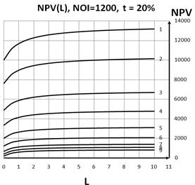
Fig. 5. Dependence of NPV on leverage level at fixed values of ![]() and
and ![]() .
.
It should be noted that this pattern should be taken into account by the Regulator which should regulate the normative base in such a way that credit rates of banks, that depends on basic rate of Central bank, not exceed, say, ![]() .
.
All curves NPV(L) at the constant values of ![]() and different values of
and different values of ![]() are started (at L=0) from one point, the higher values of
are started (at L=0) from one point, the higher values of ![]() (and lower values of
(and lower values of ![]() ) correspond to more low lying curves NPV(L). Optimum in dependence of NPV(L) is absent.
) correspond to more low lying curves NPV(L). Optimum in dependence of NPV(L) is absent.
Table 4. Dependence of NPV on leverage level S=1000 b=0.1, k0-kd=const.
| k0 | kd\L | 0.0 | 0.5 | 1.0 | 1.5 | 2.0 | 2.5 | 3.0 | 3.5 | 4.0 | 4.5 | |
| 1 | 0.08 | 0.06 | 0.0 | 285.7 | 555.6 | 818.2 | 1076.9 | 1333.3 | 1588.2 | 1842.1 | 2095.2 | 2347.8 |
| 2 | 0.10 | 0.08 | -200.0 | -57.1 | 66.7 | 181.8 | 292.3 | 400.0 | 505.9 | 610.5 | 714.3 | 817.4 |
| 3 | 0.14 | 0.12 | -428.6 | -449.0 | -492.1 | -545.5 | -604.4 | -666.7 | -731.1 | -797.0 | -863.9 | -931.7 |
| 4 | 0.18 | 0.16 | -555.6 | -666.7 | -802.5 | -949.5 | -1102.6 | -1259.3 | -1418.3 | -1578.9 | -1740.7 | -1903.4 |
| 5 | 0.24 | 0.22 | -666.7 | -857.1 | -1074.1 | -1303.0 | -1538.5 | -1777.8 | -2019.6 | -2263.2 | -2507.9 | -2753.6 |
| 6 | 0.30 | 0.28 | -733.3 | -971.4 | -1237.0 | -1515.2 | -1800.0 | -2088.9 | -2380.4 | -2673.7 | -2968.3 | -3263.8 |
| 7 | 0.36 | 0.34 | -777.8 | -1047.6 | -1345.7 | -1656.6 | -1974.4 | -2296.3 | -2620.9 | -2947.4 | -3275.1 | -3603.9 |
| 8 | 0.40 | 0.38 | -800.0 | -1085.7 | -1400.0 | -1727.3 | -2061.5 | -2400.0 | -2741.2 | -3084.2 | -3428.6 | -3773.9 |
| 9 | 0.44 | 0.42 | -818.2 | -1116.9 | -1444.4 | -1785.1 | -2132.9 | -2484.8 | -2839.6 | -3196.2 | -3554.1 | -3913.0 |
| 10 | 0.10 | 0.06 | -200.0 | 28.6 | 244.4 | 454.5 | 661.5 | 866.7 | 1070.6 | 1273.7 | 1476.2 | 1678.3 |
| 11 | 0.12 | 0.08 | -333.3 | -214.3 | -111.1 | -15.2 | 76.9 | 166.7 | 254.9 | 342.1 | 428.6 | 514.5 |
| 12 | 0.16 | 0.12 | -500.0 | -517.9 | -555.6 | -602.3 | -653.8 | -708.3 | -764.7 | -822.4 | -881.0 | -940.2 |
| 13 | 0.20 | 0.16 | -600.0 | -700.0 | -822.2 | -954.5 | -1092.3 | -1233.3 | -1376.5 | -1521.1 | -1666.7 | -1813.0 |
| 14 | 0.24 | 0.20 | -666.7 | -821.4 | -1000.0 | -1189.4 | -1384.6 | -1583.3 | -1784.3 | -1986.8 | -2190.5 | -2394.9 |
| 15 | 0.30 | 0.26 | -733.3 | -942.9 | -1177.8 | -1424.2 | -1676.9 | -1933.3 | -2192.2 | -2452.6 | -2714.3 | -2976.8 |
| 16 | 0.36 | 0.32 | -777.8 | -1023.8 | -1296.3 | -1580.8 | -1871.8 | -2166.7 | -2464.1 | -2763.2 | -3063.5 | -3364.7 |
| 17 | 0.40 | 0.36 | -800.0 | -1064.3 | -1355.6 | -1659.1 | -1969.2 | -2283.3 | -2600.0 | -2918.4 | -3238.1 | -3558.7 |
| 18 | 0.44 | 0.40 | -818.2 | -1097.4 | -1404.0 | -1723.1 | -2049.0 | -2378.8 | -2711.2 | -3045.5 | -3381.0 | -3717.4 |
Table 4. (continue)
| k0 | kd\L | 5.0 | 5.5 | 6.0 | 6.5 | 7.0 | 7.5 | 8.0 | 8.5 | 9.0 | 9.5 | 10.0 | |
| 1 | 0.08 | 0.06 | 2600.0 | 2851.9 | 3103.4 | 3354.8 | 3606.1 | 3857.1 | 4108.1 | 4359.0 | 4609.8 | 4860.5 | 5111.1 |
| 2 | 0.10 | 0.08 | 920.0 | 1022.2 | 1124.1 | 1225.8 | 1327.3 | 1428.6 | 1529.7 | 1630.8 | 1731.7 | 1832.6 | 1933.3 |
| 3 | 0.14 | 0.12 | -1000.0 | -1068.8 | -1137.9 | -1207.4 | -1277.1 | -1346.9 | -1417.0 | -1487.2 | -1557.5 | -1627.9 | -1698.4 |
| 4 | 0.18 | 0.16 | -2066.7 | -2230.5 | -2394.6 | -2559.1 | -2723.9 | -2888.9 | -3054.1 | -3219.4 | -3384.8 | -3550.4 | -3716.0 |
| 5 | 0.24 | 0.22 | -3000.0 | -3246.9 | -3494.3 | -3741.9 | -3989.9 | -4238.1 | -4486.5 | -4735.0 | -4983.7 | -5232.6 | -5481.5 |
| 6 | 0.30 | 0.28 | -3560.0 | -3856.8 | -4154.0 | -4451.6 | -4749.5 | -5047.6 | -5345.9 | -5644.4 | -5943.1 | -6241.9 | -6540.7 |
| 7 | 0.36 | 0.34 | -3933.3 | -4263.4 | -4593.9 | -4924.7 | -5255.9 | -5587.3 | -5918.9 | -6250.7 | -6582.7 | -6914.7 | -7246.9 |
| 8 | 0.40 | 0.38 | -4120.0 | -4466.7 | -4813.8 | -5161.3 | -5509.1 | -5857.1 | -6205.4 | -6553.8 | -6902.4 | -7251.2 | -7600.0 |
| 9 | 0.44 | 0.42 | -4272.7 | -4633.0 | -4993.7 | -5354.8 | -5716.3 | -6077.9 | -6439.8 | -6801.9 | -7164.1 | -7526.4 | -7888.9 |
| 10 | 0.10 | 0.06 | 1880.0 | 2081.5 | 2282.8 | 2483.9 | 2684.8 | 2885.7 | 3086.5 | 3287.2 | 3487.8 | 3688.4 | 3888.9 |
| 11 | 0.12 | 0.08 | 600.0 | 685.2 | 770.1 | 854.8 | 939.4 | 1023.8 | 1108.1 | 1192.3 | 1276.4 | 1360.5 | 1444.4 |
| 12 | 0.16 | 0.12 | -1000.0 | -1060.2 | -1120.7 | -1181.5 | -1242.4 | -1303.6 | -1364.9 | -1426.3 | -1487.8 | -1549.4 | -1611.1 |
| 13 | 0.20 | 0.16 | -1960.0 | -2107.4 | -2255.2 | -2403.2 | -2551.5 | -2700.0 | -2848.6 | -2997.4 | -3146.3 | -3295.3 | -3444.4 |
| 14 | 0.24 | 0.20 | -2600.0 | -2805.6 | -3011.5 | -3217.7 | -3424.2 | -3631.0 | -3837.8 | -4044.9 | -4252.0 | -4459.3 | -4666.7 |
| 15 | 0.30 | 0.26 | -3240.0 | -3503.7 | -3767.8 | -4032.3 | -4297.0 | -4561.9 | -4827.0 | -5092.3 | -5357.7 | -5623.3 | -5888.9 |
| 16 | 0.36 | 0.32 | -3666.7 | -3969.1 | -4272.0 | -4575.3 | -4878.8 | -5182.5 | -5486.5 | -5790.6 | -6094.9 | -6399.2 | -6703.7 |
| 17 | 0.40 | 0.36 | -3880.0 | -4201.9 | -4524.1 | -4846.8 | -5169.7 | -5492.9 | -5816.2 | -6139.7 | -6463.4 | -6787.2 | -7111.1 |
| 18 | 0.44 | 0.40 | -4054.5 | -4392.3 | -4730.4 | -5068.9 | -5407.7 | -5746.8 | -6086.0 | -6425.4 | -6765.0 | -7104.7 | -7444.4 |
3. The Effectiveness of the Investment Project from the Perspective of the Equity and Debt Owners
3.1. With the Division of Credit and Investment Flows
At a constant investment value(I = const)
![]() (5)
(5)
1) At the constant values of ![]() NPV practically always decreases with leverage. At small L values for many pairs of values
NPV practically always decreases with leverage. At small L values for many pairs of values ![]() and
and ![]() (for example,
(for example, ![]() (24%) and
(24%) and ![]() (22%) ;
(22%) ; ![]() (30%) and
(30%) and ![]() (28%) and many others there is an optimum in the dependence of NPV(L) at small
(28%) and many others there is an optimum in the dependence of NPV(L) at small ![]()
For higher values of ![]() (and, respectively,
(and, respectively, ![]() ) all curves NPV(L) lie below. With growth of NOI all curves NPV(L) are shifted parallel upwards.
) all curves NPV(L) lie below. With growth of NOI all curves NPV(L) are shifted parallel upwards.
2) At the constant values of ![]() NPV practically always decreases with leverage, passing through (most often), or not passing (more rarely) through optimum in the dependence of NPV(L) at small
NPV practically always decreases with leverage, passing through (most often), or not passing (more rarely) through optimum in the dependence of NPV(L) at small ![]()
All curves NPV(L) at the constant values of ![]() and different values of
and different values of ![]() are started (at L=0) from one point, the higher values of
are started (at L=0) from one point, the higher values of ![]() (and lower values of
(and lower values of ![]() ) correspond to higher lying curves NPV(L). With growth of NOI all curves NPV(L) are shifted practically parallel upwards.
) correspond to higher lying curves NPV(L). With growth of NOI all curves NPV(L) are shifted practically parallel upwards.
3) At the constant values of ![]() NPV practically always decreases with leverage, optimum in the dependence of NPV(L) is absent. All curves NPV(L) at the constant values of
NPV practically always decreases with leverage, optimum in the dependence of NPV(L) is absent. All curves NPV(L) at the constant values of ![]() are started (at L=0) from one point, the higher values of
are started (at L=0) from one point, the higher values of ![]() (and higher values of
(and higher values of ![]() ) correspond to lower lying curves NPV(L). With growth of NOI all curves NPV(L) are shifted practically parallel upwards.
) correspond to lower lying curves NPV(L). With growth of NOI all curves NPV(L) are shifted practically parallel upwards.
Table 5. Dependence of NPV on leverage level NOI=1200 I=2000, k0-kd=const.
| k0 | kd\L | 0.0 | 0.5 | 1.0 | 1.5 | 2.0 | 2.5 | 3.0 | 3.5 | 4.0 | 4.5 | |
| 1 | 0.08 | 0.06 | 10000.0 | 9042.4 | 8200.0 | 7470.8 | 6838.1 | 6285.7 | 5800.0 | 5369.9 | 4986.7 | 4643.1 |
| 2 | 0.10 | 0.08 | 7600.0 | 7022.2 | 6475.9 | 5981.9 | 5539.4 | 5142.9 | 4786.5 | 4465.0 | 4173.7 | 3908.7 |
| 3 | 0.14 | 0.12 | 4857.1 | 4619.8 | 4353.8 | 4093.7 | 3848.1 | 3619.0 | 3406.4 | 3209.1 | 3025.9 | 2855.6 |
| 4 | 0.18 | 0.16 | 3333.3 | 3239.7 | 3098.0 | 2945.9 | 2795.0 | 2649.4 | 2510.5 | 2378.9 | 2254.4 | 2136.8 |
| 5 | 0.24 | 0.22 | 2000.0 | 2004.3 | 1950.0 | 1876.4 | 1796.1 | 1714.3 | 1633.3 | 1554.4 | 1477.9 | 1404.2 |
| 6 | 0.30 | 0.28 | 1200.0 | 1250.2 | 1238.0 | 1203.0 | 1158.2 | 1109.2 | 1058.6 | 1007.7 | 957.4 | 907.9 |
| 7 | 0.36 | 0.34 | 666.7 | 742.0 | 753.2 | 740.0 | 715.6 | 685.7 | 652.9 | 618.8 | 584.2 | 549.5 |
| 8 | 0.40 | 0.38 | 400.0 | 486.3 | 507.7 | 504.2 | 488.9 | 467.5 | 442.9 | 416.4 | 389.0 | 361.2 |
| 9 | 0.44 | 0.42 | 181.8 | 276.2 | 305.3 | 309.0 | 300.6 | 285.7 | 267.2 | 246.6 | 224.8 | 202.3 |
| 10 | 0.10 | 0.06 | 7600.0 | 6409.2 | 5472.7 | 4726.5 | 4120.3 | 3619.0 | 3198.0 | 2839.4 | 2530.5 | 2261.7 |
| 11 | 0.12 | 0.08 | 6000.0 | 5192.2 | 4515.8 | 3954.3 | 3484.1 | 3085.7 | 2744.4 | 2449.0 | 2191.0 | 1963.6 |
| 12 | 0.16 | 0.12 | 4000.0 | 3587.9 | 3200.0 | 2855.4 | 2552.4 | 2285.7 | 2050.0 | 1840.5 | 1653.3 | 1485.2 |
| 13 | 0.20 | 0.16 | 2800.0 | 2577.8 | 2337.9 | 2111.0 | 1903.0 | 1714.3 | 1543.2 | 1388.0 | 1246.8 | 1118.0 |
| 14 | 0.24 | 0.20 | 2000.0 | 1883.3 | 1729.4 | 1573.3 | 1424.6 | 1285.7 | 1157.1 | 1038.4 | 928.7 | 827.3 |
| 15 | 0.30 | 0.26 | 1200.0 | 1171.3 | 1091.6 | 998.6 | 904.0 | 8 0 | 724.2 | 641.2 | 563.0 | 489.4 |
| 16 | 0.36 | 0.32 | 666.7 | 686.5 | 649.0 | 592.9 | 530.8 | 467.5 | 405.3 | 345.0 | 287.2 | 232.0 |
| 17 | 0.40 | 0.36 | 400.0 | 441.0 | 422.2 | 382.9 | 335.6 | 285.7 | 235.5 | 186.1 | 138.2 | 92.0 |
| 18 | 0.44 | 0.40 | 181.8 | 238.6 | 233.9 | 207.2 | 171.4 | 131.9 | 91.0 | 50.2 | 10.1 | -28.9 |
Table 5. (continue)
| k0 | kd\L | 5.0 | 5.5 | 6.0 | 6.5 | 7.0 | 7.5 | 8.0 | 8.5 | 9.0 | 9.5 | 10.0 | |
| 1 | 0.08 | 0.06 | 4333.3 | 4052.7 | 3797.4 | 3564.1 | 3350.0 | 3152.9 | 2970.9 | 2802.3 | 2645.7 | 2499.8 | 2363.6 |
| 2 | 0.10 | 0.08 | 3666.7 | 3444.8 | 3240.8 | 3052.5 | 2878.3 | 2716.6 | 2566.1 | 2425.7 | 2294.4 | 2171.4 | 2055.9 |
| 3 | 0.14 | 0.12 | 2697.0 | 2549.0 | 2410.7 | 2281.1 | 2159.5 | 2045.2 | 1937.6 | 1836.2 | 1740.3 | 1649.6 | 1563.6 |
| 4 | 0.18 | 0.16 | 2025.6 | 1920.6 | 1821.1 | 1726.9 | 1637.7 | 1552.9 | 1472.4 | 1395.9 | 1323.0 | 1253.5 | 1187.2 |
| 5 | 0.24 | 0.22 | 1333.3 | 1265.3 | 1200.0 | 1137.4 | 1077.3 | 1019.6 | 964.3 | 911.1 | 860.0 | 810.9 | 763.6 |
| 6 | 0.30 | 0.28 | 859.6 | 8 7 | 767.1 | 722.9 | 680.1 | 638.7 | 598.5 | 559.7 | 522.2 | 485.8 | 450.6 |
| 7 | 0.36 | 0.34 | 515.2 | 481.3 | 448.1 | 415.6 | 383.9 | 352.9 | 322.8 | 293.4 | 264.8 | 236.9 | 209.8 |
| 8 | 0.40 | 0.38 | 333.3 | 305.7 | 278.3 | 251.4 | 225.0 | 199.1 | 173.7 | 148.9 | 124.7 | 101.0 | 77.9 |
| 9 | 0.44 | 0.42 | 179.5 | 156.6 | 133.9 | 111.4 | 89.1 | 67.2 | 45.7 | 24.6 | 3.8 | -16.5 | -36.4 |
| 10 | 0.10 | 0.06 | 2025.6 | 1816.7 | 1630.5 | 1463.5 | 1313.0 | 1176.5 | 1052.2 | 938.5 | 834.2 | 738.1 | 649.4 |
| 11 | 0.12 | 0.08 | 1761.9 | 1581.7 | 1419.8 | 1273.5 | 1140.7 | 1019.6 | 908.7 | 806.9 | 7 9 | 626.1 | 545.5 |
| 12 | 0.16 | 0.12 | 1333.3 | 1195.6 | 1070.1 | 955.4 | 850.0 | 752.9 | 663.2 | 580.1 | 502.9 | 430.9 | 363.6 |
| 13 | 0.20 | 0.16 | 1000.0 | 891.7 | 791.8 | 699.6 | 614.2 | 534.8 | 460.8 | 391.8 | 327.2 | 266.7 | 209.8 |
| 14 | 0.24 | 0.20 | 733.3 | 646.2 | 565.1 | 489.5 | 419.0 | 352.9 | 291.0 | 232.9 | 178.2 | 126.6 | 77.9 |
| 15 | 0.30 | 0.26 | 420.3 | 355.3 | 294.1 | 236.4 | 182.1 | 130.7 | 82.2 | 36.2 | -7.3 | -48.7 | -88.0 |
| 16 | 0.36 | 0.32 | 179.5 | 129.5 | 82.0 | 36.8 | -6.2 | -47.1 | -86.0 | -123.1 | -158.5 | -192.3 | -224.6 |
| 17 | 0.40 | 0.36 | 47.6 | 5.1 | -35.5 | -74.4 | -111.5 | -147.1 | -181.0 | -213.5 | -244.7 | -274.5 | -303.0 |
| 18 | 0.44 | 0.40 | -66.7 | -103.1 | -138.2 | -171.9 | -204.2 | -235.3 | -265.1 | -293.8 | -321.3 | -347.8 | -373.2 |
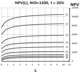
Fig. 6. Dependence of NPV on leverage level at fixed values of ![]() and
and ![]() .
.
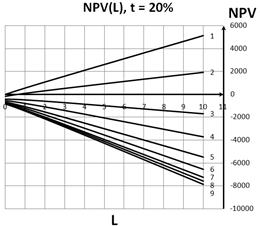
Fig. 7. Dependence of NPV on leverage level at fixed values of ![]() and
and ![]() .
.
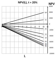
Fig. 8. Dependence of NPV on leverage level at fixed values of ![]() and
and ![]() .
.
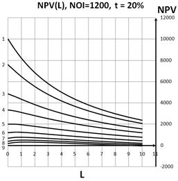
Fig. 9. Dependence of NPV on leverage level at fixed values of ![]() and
and ![]() .
.
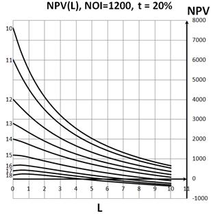
Fig. 10. Dependence of NPV on leverage level at fixed values of ![]() and
and ![]() .
.
At a constant equity value(S = const)
![]() (6)
(6)
1) At the constant values of ![]() NPV practically always decreases with leverage, optimum in the dependence of NPV(L) is absent. All curves NPV(L) at the constant values of
NPV practically always decreases with leverage, optimum in the dependence of NPV(L) is absent. All curves NPV(L) at the constant values of ![]() are started (at L=0) from one point, the higher values of
are started (at L=0) from one point, the higher values of ![]() (and, respectively,
(and, respectively, ![]() ) correspond to lower lying curves NPV(L). With growth of
) correspond to lower lying curves NPV(L). With growth of ![]() the density of curves NPV(L) increases.
the density of curves NPV(L) increases.
2) At the constant values of ![]() NPV decreases with leverage, optimum in the dependence of NPV(L) is absent. All curves NPV(L) at the constant values of
NPV decreases with leverage, optimum in the dependence of NPV(L) is absent. All curves NPV(L) at the constant values of ![]() are started (at L=0) from one point, the higher values of
are started (at L=0) from one point, the higher values of ![]() (and, respectively, the lower values of
(and, respectively, the lower values of ![]() ) correspond to higher lying curves NPV(L). With growth of
) correspond to higher lying curves NPV(L). With growth of ![]() the density of curves NPV(L) increases.
the density of curves NPV(L) increases.
3) At the constant values of ![]() NPV decreases with leverage, optimum in the dependence of NPV(L) is absent. All curves NPV(L) at the constant values of
NPV decreases with leverage, optimum in the dependence of NPV(L) is absent. All curves NPV(L) at the constant values of ![]() are started (at L=0) from one point, the higher values of
are started (at L=0) from one point, the higher values of ![]() (and, respectively, the higher values of
(and, respectively, the higher values of ![]() ) correspond to lower lying curves NPV(L). With decrease of NOI the density of curves NPV(L) increases and they are shifted down.
) correspond to lower lying curves NPV(L). With decrease of NOI the density of curves NPV(L) increases and they are shifted down.
Table 6. Dependence of NPV on leverage level NOI=1200 I=2000, k0-kd=const.
| k0 | kd\L | 0.0 | 0.5 | 1.0 | 1.5 | 2.0 | 2.5 | 3.0 | 3.5 | 4.0 | 4.5 | |
| 1 | 0.08 | 0.06 | 10000.0 | 8907.3 | 7828.6 | 6762.8 | 5709.1 | 4666.7 | 3634.8 | 26 8 | 1600.0 | 595.9 |
| 2 | 0.10 | 0.08 | 7600.0 | 6611.8 | 5630.8 | 4656.6 | 3688.9 | 2727.3 | 1771.4 | 821.1 | -124.1 | -1064.4 |
| 3 | 0.14 | 0.12 | 4857.1 | 3960.6 | 3066.7 | 2175.3 | 1286.5 | 400.0 | -484.2 | -1366.2 | -2246.2 | -3124.1 |
| 4 | 0.18 | 0.16 | 3333.3 | 2474.7 | 1617.4 | 761.3 | -93.6 | -947.4 | -1800.0 | -2651.5 | -3502.0 | -4351.5 |
| 5 | 0.24 | 0.22 | 2000.0 | 1166.9 | 334.4 | -497.6 | -1329.0 | -2160.0 | -2990.5 | -3820.5 | -4650.0 | -5479.1 |
| 6 | 0.30 | 0.28 | 1200.0 | 378.8 | -442.1 | -1262.7 | -2083.1 | -2903.2 | -3723.1 | -4542.7 | -5362.0 | -6181.1 |
| 7 | 0.36 | 0.34 | 666.7 | -148.1 | -962.6 | -1777.0 | -2591.3 | -3405.4 | -4219.4 | -5033.2 | -5846.8 | -6660.3 |
| 8 | 0.40 | 0.38 | 400.0 | -411.9 | -1223.8 | -2035.5 | -2847.1 | -3658.5 | -4469.9 | -5281.2 | -6092.3 | -6903.3 |
| 9 | 0.44 | 0.42 | 181.8 | -628.1 | -1437.8 | -2247.5 | -3057.1 | -3866.7 | -4676.1 | -5485.5 | -6294.7 | -7103.9 |
| 10 | 0.10 | 0.06 | 7600.0 | 6430.8 | 5288.9 | 4171.4 | 3075.9 | 2000.0 | 941.9 | -100.0 | -1127.3 | -2141.2 |
| 11 | 0.12 | 0.08 | 6000.0 | 4941.9 | 3900.0 | 2872.7 | 1858.8 | 857.1 | -133.3 | -1113.5 | -2084.2 | -3046.2 |
| 12 | 0.16 | 0.12 | 4000.0 | 3053.7 | 2114.3 | 1181.4 | 254.5 | -666.7 | -1582.6 | -2493.6 | -3400.0 | -4302.0 |
| 13 | 0.20 | 0.16 | 2800.0 | 1905.9 | 1015.4 | 128.3 | -755.6 | -1636.4 | -2514.3 | -3389.5 | -4262.1 | -5132.2 |
| 14 | 0.24 | 0.20 | 2000.0 | 1134.4 | 271.0 | -590.5 | -1450.0 | -2307.7 | -3163.6 | -4017.9 | -4870.6 | -5721.7 |
| 15 | 0.30 | 0.26 | 1200.0 | 357.9 | -483.1 | -1323.1 | -2162.0 | -3000.0 | -3837.0 | -4673.2 | -5508.4 | -6342.9 |
| 16 | 0.36 | 0.32 | 666.7 | -162.6 | -991.3 | -1819.4 | -2646.8 | -3473.7 | -4300.0 | -5125.8 | -5951.0 | -6775.8 |
| 17 | 0.40 | 0.36 | 400.0 | -423.8 | -1247.1 | -2069.9 | -2892.3 | -3714.3 | -4535.8 | -5357.0 | -6177.8 | -6998.2 |
| 18 | 0.44 | 0.40 | 181.8 | -637.8 | -1457.1 | -2276.1 | -3094.7 | -3913.0 | -4731.0 | -5548.7 | -6366.1 | -7183.2 |
Table 6. (continue)
| k0 | kd\L | 5.0 | 5.5 | 6.0 | 6.5 | 7.0 | 7.5 | 8.0 | 8.5 | 9.0 | 9.5 | 10.0 | |
| 1 | 0.08 | 0.06 | -400.0 | -1388.2 | -2369.2 | -3343.4 | -4311.1 | -5272.7 | -6228.6 | -7178.9 | -8124.1 | -9064.4 | -10000.0 |
| 2 | 0.10 | 0.08 | -2000.0 | -2931.1 | -3858.1 | -4781.0 | -5700.0 | -6615.4 | -7527.3 | -8435.8 | -9341.2 | -10243.5 | -11142.9 |
| 3 | 0.14 | 0.12 | -4000.0 | -4874.1 | -5746.3 | -6616.9 | -7485.7 | -8352.9 | -9218.6 | -10082.8 | -10945.5 | -11806.7 | -12666.7 |
| 4 | 0.18 | 0.16 | -5200.0 | -6047.5 | -6894.1 | -7739.8 | -8584.6 | -9428.6 | -10271.7 | -11114.0 | -11955.6 | -12796.3 | -13636.4 |
| 5 | 0.24 | 0.22 | -6307.7 | -7135.9 | -7963.6 | -8791.0 | -9617.9 | -10444.4 | -11270.6 | -12096.4 | -12921.7 | -13746.8 | -14571.4 |
| 6 | 0.30 | 0.28 | -7000.0 | -7818.6 | -8637.0 | -9455.2 | -10273.2 | -11090.9 | -11908.4 | -12725.7 | -13542.9 | -14359.8 | -15176.5 |
| 7 | 0.36 | 0.34 | -7473.7 | -8286.9 | -9100.0 | -9913.0 | -10725.8 | -11538.5 | -12351.0 | -13163.5 | -13975.8 | -14787.9 | -15600.0 |
| 8 | 0.40 | 0.38 | -7714.3 | -8525.1 | -9335.8 | -10146.5 | -10957.0 | -11767.4 | -12577.8 | -13388.0 | -14198.2 | -15008.2 | -15818.2 |
| 9 | 0.44 | 0.42 | -7913.0 | -8722.1 | -9531.0 | -10339.9 | -11148.7 | -11957.4 | -12766.1 | -13574.7 | -14383.2 | -15191.6 | -16000.0 |
| 10 | 0.10 | 0.06 | -3142.9 | -4133.3 | -5113.5 | -6084.2 | -7046.2 | -8000.0 | -8946.3 | -9885.7 | -10818.6 | -11745.5 | -12666.7 |
| 11 | 0.12 | 0.08 | -4000.0 | -4946.3 | -5885.7 | -6818.6 | -7745.5 | -8666.7 | -9582.6 | -10493.6 | -11400.0 | -12302.0 | -13200.0 |
| 12 | 0.16 | 0.12 | -5200.0 | -6094.1 | -6984.6 | -7871.7 | -8755.6 | -9636.4 | -10514.3 | -11389.5 | -12262.1 | -13132.2 | -14000.0 |
| 13 | 0.20 | 0.16 | -6000.0 | -6865.6 | -7729.0 | -8590.5 | -9450.0 | -10307.7 | -11163.6 | -12017.9 | -12870.6 | -13721.7 | -14571.4 |
| 14 | 0.24 | 0.20 | -6571.4 | -7419.7 | -8266.7 | -91 3 | -9956.8 | -10800.0 | -11642.1 | -12483.1 | -13323.1 | -14162.0 | -15000.0 |
| 15 | 0.30 | 0.26 | -7176.5 | -8009.3 | -8841.4 | -9672.7 | -10503.4 | -11333.3 | -12162.6 | -12991.3 | -13819.4 | -14646.8 | -15473.7 |
| 16 | 0.36 | 0.32 | -7600.0 | -8423.8 | -9247.1 | -10069.9 | -10892.3 | -11714.3 | -12535.8 | -13357.0 | -14177.8 | -14998.2 | -15818.2 |
| 17 | 0.40 | 0.36 | -7818.2 | -8637.8 | -9457.1 | -10276.1 | -11094.7 | -11913.0 | -12731.0 | -13548.7 | -14366.1 | -15183.2 | -16000.0 |
| 18 | 0.44 | 0.40 | -8000.0 | -8816.5 | -9632.8 | -10448.8 | -11264.5 | -12080.0 | -12895.2 | -13710.2 | -14525.0 | -15339.5 | -16153.8 |
3.2. Without Flows Separation
At a constant investment value(I = const)
 (7)
(7)
At the constant values of ![]() NPV demonstrates a limited growth with leverage with output into saturation regime. The main increase in NPV occurs when
NPV demonstrates a limited growth with leverage with output into saturation regime. The main increase in NPV occurs when ![]() . With growth of
. With growth of ![]() (and
(and ![]() ) the сurves NPV(L) are lowered. Optimum in the dependence of NPV(L) is absent.
) the сurves NPV(L) are lowered. Optimum in the dependence of NPV(L) is absent.
With growth of NOI all curves NPV(L) are shifted practically parallel upwards.
2) At the constant values of ![]() NPV demonstrates a limited growth with leverage with output into saturation regime. All curves NPV(L) at the constant values of
NPV demonstrates a limited growth with leverage with output into saturation regime. All curves NPV(L) at the constant values of ![]() and different values of
and different values of ![]() are started (at L=0) from one point, the higher values of
are started (at L=0) from one point, the higher values of ![]() (and, respectively the lower values of
(and, respectively the lower values of ![]() ) correspond to higher lying curves NPV(L). Optimum in the dependence of NPV(L) is absent. With growth of NOI all curves NPV(L) are shifted practically parallel upwards.
) correspond to higher lying curves NPV(L). Optimum in the dependence of NPV(L) is absent. With growth of NOI all curves NPV(L) are shifted practically parallel upwards.
Fig. 11. Dependence of NPV on leverage level at fixed values of ![]() and
and ![]() .
.
3) At the constant values of ![]() NPV shows a limited growth with leverage with output into saturation regime. All curves NPV(L) at the constant values of
NPV shows a limited growth with leverage with output into saturation regime. All curves NPV(L) at the constant values of ![]() and different values of
and different values of ![]() are started (at L=0) from one point, the higher values of
are started (at L=0) from one point, the higher values of ![]() (and, respectively, the higher values of
(and, respectively, the higher values of ![]() ) correspond to lower lying curves NPV(L). Optimum in the dependence of NPV(L) is absent.
) correspond to lower lying curves NPV(L). Optimum in the dependence of NPV(L) is absent.
Table 7. Dependence of NPV on leverage level NOI=1200 I=2000, k0-kd=const.
| k0 | kd\L | 0.0 | 0.5 | 1.0 | 1.5 | 2.0 | 2.5 | 3.0 | 3.5 | 4.0 | 4.5 | |
| 1 | 0.08 | 0.06 | 10000.0 | 10964.3 | 11500.0 | 11840.9 | 12076.9 | 12250.0 | 12382.4 | 12486.8 | 12571.4 | 12641.3 |
| 2 | 0.10 | 0.08 | 7600.0 | 8400.0 | 8844.4 | 9127.3 | 9323.1 | 9466.7 | 9576.5 | 9663.2 | 9733.3 | 9791.3 |
| 3 | 0.14 | 0.12 | 4857.1 | 5469.4 | 5809.5 | 6026.0 | 6175.8 | 6285.7 | 6369.7 | 6436.1 | 6489.8 | 6534.2 |
| 4 | 0.18 | 0.16 | 3333.3 | 3841.3 | 4123.5 | 4303.0 | 4427.4 | 4518.5 | 4588.2 | 4643.3 | 4687.8 | 4724.6 |
| 5 | 0.24 | 0.22 | 2000.0 | 2416.7 | 2648.1 | 2795.5 | 2897.4 | 2972.2 | 3029.4 | 3074.6 | 3111.1 | 3141.3 |
| 6 | 0.30 | 0.28 | 1200.0 | 1561.9 | 1763.0 | 1890.9 | 1979.5 | 2044.4 | 2094.1 | 2133.3 | 2165.1 | 2191.3 |
| 7 | 0.36 | 0.34 | 666.7 | 992.1 | 1172.8 | 1287.9 | 1367.5 | 1425.9 | 1470.6 | 1505.8 | 1534.4 | 1558.0 |
| 8 | 0.40 | 0.38 | 400.0 | 707.1 | 877.8 | 986.4 | 1061.5 | 1116.7 | 1158.8 | 1192.1 | 1219.0 | 1241.3 |
| 9 | 0.44 | 0.42 | 181.8 | 474.0 | 636.4 | 739.7 | 811.2 | 863.6 | 903.7 | 935.4 | 961.0 | 982.2 |
| 10 | 0.10 | 0.06 | 7600.0 | 8371.4 | 8800.0 | 9072.7 | 9261.5 | 9400.0 | 9505.9 | 9589.5 | 9657.1 | 9713.0 |
| 11 | 0.12 | 0.08 | 6000.0 | 6666.7 | 7037.0 | 7272.7 | 7435.9 | 7555.6 | 7647.1 | 7719.3 | 7777.8 | 7826.1 |
| 12 | 0.16 | 0.12 | 4000.0 | 4535.7 | 4833.3 | 5022.7 | 5153.8 | 5250.0 | 5323.5 | 5381.6 | 5428.6 | 5467.4 |
| 13 | 0.20 | 0.16 | 2800.0 | 3257.1 | 3511.1 | 3672.7 | 3784.6 | 3866.7 | 3929.4 | 3978.9 | 4019.0 | 4052.2 |
| 14 | 0.24 | 0.20 | 2000.0 | 2404.8 | 2629.6 | 2772.7 | 2871.8 | 2944.4 | 3000.0 | 3043.9 | 3079.4 | 3108.7 |
| 15 | 0.30 | 0.26 | 1200.0 | 1552.4 | 1748.1 | 1872.7 | 1959.0 | 2022.2 | 2070.6 | 2108.8 | 2139.7 | 2165.2 |
| 16 | 0.36 | 0.32 | 666.7 | 984.1 | 1160.5 | 1272.7 | 1350.4 | 1407.4 | 1451.0 | 1485.4 | 1513.2 | 1536.2 |
| 17 | 0.40 | 0.36 | 400.0 | 700.0 | 866.7 | 972.7 | 1046.2 | 1100.0 | 1141.2 | 1173.7 | 1200.0 | 1221.7 |
| 18 | 0.44 | 0.40 | 181.8 | 467.5 | 626.3 | 727.3 | 797.2 | 848.5 | 887.7 | 918.7 | 943.7 | 964.4 |
Table 7. (continue)
| k0 | kd\L | 5.0 | 5.5 | 6.0 | 6.5 | 7.0 | 7.5 | 8.0 | 8.5 | 9.0 | 9.5 | 10.0 | |
| 1 | 0.08 | 0.06 | 12700.0 | 12750.0 | 12793.1 | 12830.6 | 12863.6 | 12892.9 | 12918.9 | 12942.3 | 12963.4 | 12982.6 | 13000.0 |
| 2 | 0.10 | 0.08 | 9840.0 | 9881.5 | 9917.2 | 9948.4 | 9975.8 | 10000.0 | 10021.6 | 10041.0 | 10058.5 | 10074.4 | 10088.9 |
| 3 | 0.14 | 0.12 | 6571.4 | 6603.2 | 6630.5 | 6654.4 | 6675.3 | 6693.9 | 6710.4 | 6725.3 | 6738.7 | 6750.8 | 6761.9 |
| 4 | 0.18 | 0.16 | 4755.6 | 4781.9 | 4804.6 | 4824.4 | 4841.8 | 4857.1 | 4870.9 | 4883.2 | 4894.3 | 4904.4 | 4913.6 |
| 5 | 0.24 | 0.22 | 3166.7 | 3188.3 | 3206.9 | 3223.1 | 3237.4 | 3250.0 | 3261.3 | 3271.4 | 3280.5 | 3288.8 | 3296.3 |
| 6 | 0.30 | 0.28 | 2213.3 | 2232.1 | 2248.3 | 2262.4 | 2274.7 | 2285.7 | 2295.5 | 2304.3 | 23 2 | 2319.4 | 2325.9 |
| 7 | 0.36 | 0.34 | 1577.8 | 1594.7 | 1609.2 | 1621.9 | 1633.0 | 1642.9 | 1651.7 | 1659.5 | 1666.7 | 1673.1 | 1679.0 |
| 8 | 0.40 | 0.38 | 1260.0 | 1275.9 | 1289.7 | 1301.6 | 13 1 | 1321.4 | 1329.7 | 1337.2 | 1343.9 | 1350.0 | 1355.6 |
| 9 | 0.44 | 0.42 | 1000.0 | 1015.2 | 1028.2 | 1039.6 | 1049.6 | 1058.4 | 1066.3 | 1073.4 | 1079.8 | 1085.6 | 1090.9 |
| 10 | 0.10 | 0.06 | 9760.0 | 9800.0 | 9834.5 | 9864.5 | 9890.9 | 9914.3 | 9935.1 | 9953.8 | 9970.7 | 9986.0 | 10000.0 |
| 11 | 0.12 | 0.08 | 7866.7 | 7901.2 | 7931.0 | 7957.0 | 7979.8 | 8000.0 | 8018.0 | 8034.2 | 8048.8 | 8062.0 | 8074.1 |
| 12 | 0.16 | 0.12 | 5500.0 | 5527.8 | 5551.7 | 5572.6 | 5590.9 | 5607.1 | 5621.6 | 5634.6 | 5646.3 | 5657.0 | 5666.7 |
| 13 | 0.20 | 0.16 | 4080.0 | 4103.7 | 4124.1 | 4141.9 | 4157.6 | 4171.4 | 4183.8 | 4194.9 | 4204.9 | 4214.0 | 4222.2 |
| 14 | 0.24 | 0.20 | 3133.3 | 3154.3 | 3172.4 | 3188.2 | 3202.0 | 3214.3 | 3225.2 | 3235.0 | 3243.9 | 3251.9 | 3259.3 |
| 15 | 0.30 | 0.26 | 2186.7 | 2204.9 | 2220.7 | 2234.4 | 2246.5 | 2257.1 | 2266.7 | 2275.2 | 2282.9 | 2289.9 | 2296.3 |
| 16 | 0.36 | 0.32 | 1555.6 | 1572.0 | 1586.2 | 1598.6 | 1609.4 | 1619.0 | 1627.6 | 1635.3 | 1642.3 | 1648.6 | 1654.3 |
| 17 | 0.40 | 0.36 | 1240.0 | 1255.6 | 1269.0 | 1280.6 | 1290.9 | 1300.0 | 1308.1 | 1315.4 | 1322.0 | 1327.9 | 1333.3 |
| 18 | 0.44 | 0.40 | 981.8 | 996.6 | 1009.4 | 1020.5 | 1030.3 | 1039.0 | 1046.7 | 1053.6 | 1059.9 | 1065.5 | 1070.7 |
At a constant equity value (S = const)
![]() , (8)
, (8)
 . (9)
. (9)
1. At the constant values of ![]() NPV shows as an unlimited growth with leverage and unlimited descending with leverage. It is interesting to note, that the credit rate value
NPV shows as an unlimited growth with leverage and unlimited descending with leverage. It is interesting to note, that the credit rate value ![]() turns out to be a border at all surveyed values of
turns out to be a border at all surveyed values of ![]() , equal to 2%, 4%, 6%, 10% (it separates the growth of NPV with leverage from descending of NPV with leverage). In other words, with growth of
, equal to 2%, 4%, 6%, 10% (it separates the growth of NPV with leverage from descending of NPV with leverage). In other words, with growth of ![]() the transition from the growth of NPV with leverage to its descending with leverage takes place, and at the credit rate
the transition from the growth of NPV with leverage to its descending with leverage takes place, and at the credit rate ![]() NPV does not depends on the leverage level at all surveyed values of
NPV does not depends on the leverage level at all surveyed values of ![]() .
.
Thus, we come to conclusion, that for perpetuity projects NPV grows with leverage at a credit rate ![]() and NPV decreases with leverage at a credit rate
and NPV decreases with leverage at a credit rate ![]() (project remains effective up to leverage levels
(project remains effective up to leverage levels ![]() ,
, ![]() ). Optimum in the dependence of NPV(L) is absent.
). Optimum in the dependence of NPV(L) is absent.
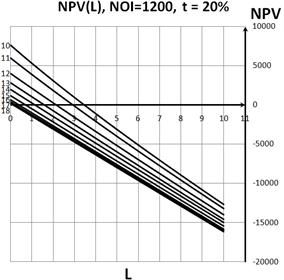
Fig. 12. Dependence of NPV on leverage level at fixed values of ![]() and
and ![]() .
.
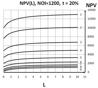
Fig. 13. Dependence of NPV on leverage level at fixed values of ![]() and
and ![]() .
.
2. At the constant values of ![]() NPV shows an unlimited growth with leverage as well as unlimited descending with leverage. NPV grows with leverage at a credit rate
NPV shows an unlimited growth with leverage as well as unlimited descending with leverage. NPV grows with leverage at a credit rate ![]() and NPV decreases with leverage at a credit rate
and NPV decreases with leverage at a credit rate ![]() (project remains effective up to leverage levels
(project remains effective up to leverage levels ![]() ,
, ![]() ). All curves NPV(L) at the constant values of
). All curves NPV(L) at the constant values of ![]() and different values of
and different values of ![]() are started (at L=0) from one point, the higher values of
are started (at L=0) from one point, the higher values of ![]() (and higher values of
(and higher values of ![]() ) correspond to more low lying curves NPV(L). Optimum in dependence of NPV(L) is absent.
) correspond to more low lying curves NPV(L). Optimum in dependence of NPV(L) is absent.
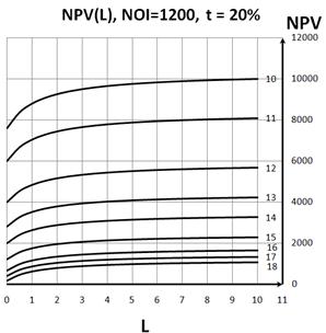
Fig. 14. Dependence of NPV on leverage level at fixed values of ![]() and
and ![]() .
.
3. At the constant values of ![]() NPV as well as in case of constant values of
NPV as well as in case of constant values of ![]() shows mainly an unlimited growth with leverage. Unlimited descending with leverage was shown for the pair
shows mainly an unlimited growth with leverage. Unlimited descending with leverage was shown for the pair ![]() only. All curves NPV(L) at the constant values of
only. All curves NPV(L) at the constant values of ![]() and different values of
and different values of ![]() are started (at L=0) from one point, the higher values of
are started (at L=0) from one point, the higher values of ![]() (and lower values of
(and lower values of ![]() ) correspond to more high lying curves NPV(L). Optimum in dependence of NPV(L) is absent.
) correspond to more high lying curves NPV(L). Optimum in dependence of NPV(L) is absent.
Table 8. Dependence of NPV on leverage level S=1000 b=0.1, k0-kd=const.
| k0 | kd\L | 0.0 | 0.5 | 1.0 | 1.5 | 2.0 | 2.5 | 3.0 | 3.5 | 4.0 | 4.5 | |
| 1 | 0.08 | 0.06 | 0.0 | 187.5 | 388.9 | 596.6 | 807.7 | 1020.8 | 1235.3 | 1450.7 | 1666.7 | 1883.2 |
| 2 | 0.10 | 0.08 | -200.0 | -128.6 | -44.4 | 45.5 | 138.5 | 233.3 | 329.4 | 426.3 | 523.8 | 621.7 |
| 3 | 0.14 | 0.12 | -428.6 | -489.8 | -539.7 | -584.4 | -626.4 | -666.7 | -705.9 | -744.4 | -782.3 | -819.9 |
| 4 | 0.18 | 0.16 | -555.6 | -690.5 | -814.8 | -934.3 | -1051.3 | -1166.7 | -1281.0 | -1394.7 | -1507.9 | -1620.8 |
| 5 | 0.24 | 0.22 | -666.7 | -866.1 | -1055.6 | -1240.5 | -1423.1 | -1604.2 | -1784.3 | -1963.8 | -2142.9 | -2321.6 |
| 6 | 0.30 | 0.28 | -733.3 | -971.4 | -1200.0 | -1424.2 | -1646.2 | -1866.7 | -2086.3 | -2305.3 | -2523.8 | -2742.0 |
| 7 | 0.36 | 0.34 | -777.8 | -1041.7 | -1296.3 | -1546.7 | -1794.9 | -2041.7 | -2287.6 | -2532.9 | -2777.8 | -3022.3 |
| 8 | 0.40 | 0.38 | -800.0 | -1076.8 | -1344.4 | -1608.0 | -1869.2 | -2129.2 | -2388.2 | -2646.7 | -2904.8 | -3162.5 |
| 9 | 0.44 | 0.42 | -818.2 | -1105.5 | -1383.8 | -1658.1 | -1930.1 | -2200.8 | -2470.6 | -2739.8 | -3008.7 | -3277.2 |
| 10 | 0.10 | 0.06 | -200.0 | -150.0 | -88.9 | -22.7 | 46.2 | 116.7 | 188.2 | 260.5 | 333.3 | 406.5 |
| 11 | 0.12 | 0.08 | -333.3 | -357.1 | -370.4 | -378.8 | -384.6 | -388.9 | -392.2 | -394.7 | -396.8 | -398.6 |
| 12 | 0.16 | 0.12 | -500.0 | -616.1 | -722.2 | -823.9 | -923.1 | -1020.8 | -1117.6 | -1213.8 | -1309.5 | -1404.9 |
| 13 | 0.20 | 0.16 | -600.0 | -771.4 | -933.3 | -1090.9 | -1246.2 | -1400.0 | -1552.9 | -1705.3 | -1857.1 | -2008.7 |
| 14 | 0.24 | 0.20 | -666.7 | -875.0 | -1074.1 | -1268.9 | -1461.5 | -1652.8 | -1843.1 | -2032.9 | -2222.2 | -2411.2 |
| 15 | 0.30 | 0.26 | -733.3 | -978.6 | -1214.8 | -1447.0 | -1676.9 | -1905.6 | -2133.3 | -2360.5 | -2587.3 | -2813.8 |
| 16 | 0.36 | 0.32 | -777.8 | -1047.6 | -1308.6 | -1565.7 | -1820.5 | -2074.1 | -2326.8 | -2578.9 | -2830.7 | -3082.1 |
| 17 | 0.40 | 0.36 | -800.0 | -1082.1 | -1355.6 | -1625.0 | -1892.3 | -2158.3 | -2423.5 | -2688.2 | -2952.4 | -3216.3 |
| 18 | 0.44 | 0.40 | -818.2 | -1110.4 | -1393.9 | -1673.6 | -1951.0 | -2227.3 | -2502.7 | -2777.5 | -3051.9 | -3326.1 |
Table 8. (continue)
| k0 | kd\L | 5.0 | 5.5 | 6.0 | 6.5 | 7.0 | 7.5 | 8.0 | 8.5 | 9.0 | 9.5 | 10.0 | |
| 1 | 0.08 | 0.06 | 2100.0 | 2317.1 | 2534.5 | 2752.0 | 2969.7 | 3187.5 | 3405.4 | 3623.4 | 3841.5 | 4059.6 | 4277.8 |
| 2 | 0.10 | 0.08 | 720.0 | 818.5 | 917.2 | 1016.1 | 1115.2 | 1214.3 | 1313.5 | 14 8 | 15 2 | 1611.6 | 1711.1 |
| 3 | 0.14 | 0.12 | -857.1 | -894.2 | -931.0 | -967.7 | -1004.3 | -1040.8 | -1077.2 | -1113.6 | -1149.8 | -1186.0 | -1222.2 |
| 4 | 0.18 | 0.16 | -1733.3 | -1845.7 | -1957.9 | -2069.9 | -2181.8 | -2293.7 | -2405.4 | -2517.1 | -2628.7 | -2740.3 | -2851.9 |
| 5 | 0.24 | 0.22 | -2500.0 | -2678.2 | -2856.3 | -3034.3 | -32 1 | -3389.9 | -3567.6 | -3745.2 | -3922.8 | -4100.3 | -4277.8 |
| 6 | 0.30 | 0.28 | -2960.0 | -3177.8 | -3395.4 | -36 9 | -3830.3 | -4047.6 | -4264.9 | -4482.1 | -4699.2 | -4916.3 | -5133.3 |
| 7 | 0.36 | 0.34 | -3266.7 | -3510.8 | -3754.8 | -3998.7 | -4242.4 | -4486.1 | -4729.7 | -4973.3 | -5216.8 | -5460.3 | -5703.7 |
| 8 | 0.40 | 0.38 | -3420.0 | -3677.3 | -3934.5 | -4191.5 | -4448.5 | -4705.4 | -4962.2 | -5218.9 | -5475.6 | -5732.3 | -5988.9 |
| 9 | 0.44 | 0.42 | -3545.5 | -3813.6 | -4081.5 | -4349.3 | -4617.1 | -4884.7 | -5152.3 | -5419.9 | -5687.4 | -5954.8 | -6222.2 |
| 10 | 0.10 | 0.06 | 480.0 | 553.7 | 627.6 | 701.6 | 775.8 | 850.0 | 924.3 | 998.7 | 1073.2 | 1147.7 | 1222.2 |
| 11 | 0.12 | 0.08 | -400.0 | -401.2 | -402.3 | -403.2 | -404.0 | -404.8 | -405.4 | -406.0 | -406.5 | -407.0 | -407.4 |
| 12 | 0.16 | 0.12 | -1500.0 | -1594.9 | -1689.7 | -1784.3 | -1878.8 | -1973.2 | -2067.6 | -2161.9 | -2256.1 | -2350.3 | -2444.4 |
| 13 | 0.20 | 0.16 | -2160.0 | -2311.1 | -2462.1 | -26 9 | -2763.6 | -2914.3 | -3064.9 | -3215.4 | -3365.9 | -3516.3 | -3666.7 |
| 14 | 0.24 | 0.20 | -2600.0 | -2788.6 | -2977.0 | -3165.3 | -3353.5 | -3541.7 | -3729.7 | -3917.7 | -4105.7 | -4293.6 | -4481.5 |
| 15 | 0.30 | 0.26 | -3040.0 | -3266.0 | -3492.0 | -3717.7 | -3943.4 | -4169.0 | -4394.6 | -4620.1 | -4845.5 | -5070.9 | -5296.3 |
| 16 | 0.36 | 0.32 | -3333.3 | -3584.4 | -3835.2 | -4086.0 | -4336.7 | -4587.3 | -4837.8 | -5088.3 | -5338.8 | -5589.1 | -5839.5 |
| 17 | 0.40 | 0.36 | -3480.0 | -3743.5 | -4006.9 | -4270.2 | -4533.3 | -4796.4 | -5059.5 | -5322.4 | -5585.4 | -5848.3 | -6111.1 |
| 18 | 0.44 | 0.40 | -3600.0 | -3873.7 | -4147.3 | -4420.8 | -4694.2 | -4967.5 | -5240.8 | -5514.0 | -5787.1 | -6060.3 | -6333.3 |
4. Conclusions
We conduct the analysis of effectiveness of investment projects within the perpetuity (Modigliani–Miller) approximation (Modigliani et al 1958, 1963, 1966). Based on the obtained in previous papers results for NPV (Brusov et al 2011a,b,c,d,e; 2012 a, b; 2013 a, b, c; 2014 a, b; Filatova et al 2008) we have analyzed the effectiveness of investment projects for three cases:
1) at a constant difference between equity cost (at ![]() ) and debt cost
) and debt cost ![]() ;
;
2) at a constant equity cost (at ![]() ) and varying debt cost
) and varying debt cost ![]() ;
;
3) at a constant debt cost ![]() and varying equity cost (at
and varying equity cost (at ![]() )
) ![]()
The dependence of NPV on investment value and/or equity value will be also analyzed. The results are shown in the form of tables and graphs.
The obtained tables have played an important practical role in determining of the optimal, or acceptable debt level, at which the project remains effective. The optimal debt level there is for the situation, when in the dependence of NPV on leverage level L there is an optimum (leverage level value, at which NPV reaches a maximum value. An acceptable debt level there is for the situation, when NPV decreases with leverage. And, finally, it is possible that NPV is growing with leverage. In this case, an increase in borrowing leads to increased effectiveness of investment projects, and their limit is determined by financial sustainability of investing company.
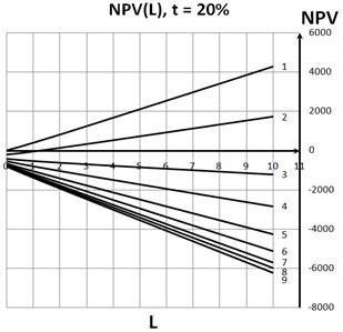
Fig. 15. Dependence of NPV on leverage level at fixed values of ![]() and
and ![]() .
.
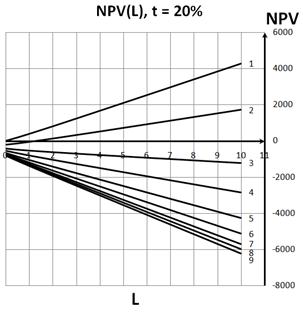
Fig. 16. Dependence of NPV on leverage level at fixed values of ![]() and
and ![]() .
.
References
- Brusov P, Filatova T, Orehova N, Eskindarov M (2015), Modern corporate finance, investments and taxation, monograph,Springer International Publishing, Switzerland, 373 p.
- Brusov P, Filatova T, Orehova N, Brusova A (2011a) Weighted average cost of capital in the theory of Modigliani–Miller, modified for a finite life–time company. Applied Financial Economics 21(11): 815-824.
- Brusov P, Filatova P, Orekhova N (2013a) Absence of an Optimal Capital Structure in the Famous Tradeoff Theory! Journal of Reviews on Global Economics 2: 94-116.
- Brusov P, Filatova P, Orekhova N (2014a) Mechanism of formation of the company optimal capital structure, different from suggested by trade off theory. Cogent Economics & Finance 2: 1-13 http://dx.doi.org/10.1080/23322039.2014.946150.
- Brusov P, Filatova T, Orehova N et al. (2011b) From Modigliani–Miller to general theory of capital cost and capital structure of the company. Research Journal of Economics, Business and ICT 2: 16–21.
- Brusov P, Filatova T, Eskindarov M, Orehova N (2012a) Influence of debt financing on the effectiveness of the finite duration investment project. Applied Financial Economics 22 (13) : 1043-1052.
- Brusov P, Filatova T, Orehova N et al (2011c) Influence of debt financing on the effectiveness of the investment project within the Modigliani–Miller theory. Research Journal of Economics, Business and ICT (UK) 2: 11-15.
- Brusov P, Filatova T, Eskindarov M, Orehova N (2012b) Hidden global causes of the global financial crisis. Journal of Reviews on Global Economics 1: 106-111.
- Brusov P, Filatova T, Orekhova N (2013b) Absence of an Optimal Capital Structure in the Famous Tradeoff Theory! Journal of Reviews on Global Economics 2: 94–116.
- Brusov P.N., Filatova Т. V. (2011d) From Modigliani–Miller to general theory of capital cost and capital structure of the company.Finance and credit 435: 2–8.
- Brusov P Filatova T Orehova N Brusov P.P Brusova N. (2011e) From Modigliani–Miller to general theory of capital cost and capital structure of the company. Research Journal of Economics, Business and ICT 2: 16–21.
- Brusov P Filatova T Orehova N (2014b) Inflation in Brusov–Filatova–Orekhova Theory and in its Perpetuity Limit – Modigliani – Miller Theory. Journal of Reviews on Global Economics 3: 175-185.
- Brusov P Filatova T Orehova N (2013c) A Qualitatively New Effect in Corporative Finance: Abnormal Dependence of Cost of Equity of Company on Leverage. Journal of Reviews on Global Economics 2: 183-193.
- Filatova Т Orehova N Brusova А (2008) Weighted average cost of capital in the theory of Modigliani–Miller, modified for a finite life–time company. Bulletin of the FU 48: 68–77.
- Brusova A (2011) А Comparison of the three methods of estimation of weighted average cost of capital and equity cost of company. Financial analysis: problems and solutions 34 (76): 36-42.
- Мodigliani F, Мiller M (1958) The Cost of Capital, Corporate Finance, and the Theory of Investment. American Economic Review 48: 261–297.
- Мodigliani F, Мiller M (1963) Corporate Income Taxes and the Cost of Capital: A Correction. American Economic Review 53: 147–175
- Modigliani F, Miller M (1966) Some estimates of the Cost of Capital to the Electric Utility Industry 1954–1957. American Economic Review 56: 333-391.


