
American Journal of Renewable and Sustainable Energy, Vol. 1, No. 1, May 2015 Publish Date: May 6, 2015 Pages: 9-15
Comparative Numerical Study of Turbulence Models for Analysis a Commercial HAWT Performance
Mojtaba Tahani1, *, Hamid Hosseinzadegan2, Mohsen Moradi1
1Faculty of New Sciences and Technologies, University of Tehran, Tehran, Iran
2Department of Mechanical Engineering, Virginia Polytechnic Institute and State University, Blacksburg, VA, USA
Abstract
In the present work, four turbulence models and their precision on results for twenty-two cases of different wind speeds, ranging from cut-in to cut-off values, and associated mean pitch angles of blades are investigated numerically. The results of 3D finite volume simulations of airflow around a commercial Vestas V80 horizontal axis wind turbine (HAWT), with a rated output power of 2 MW, are presented. The grid used in the simulations consists of two main parts i.e. unstructured mesh rotating with blades and structured hexahedral stationary one for the external domain. Several cases with different free stream velocities (and different tip speed ratios and mean pitch angles) are studied, employing four different turbulence models: ![]() SST,
SST, ![]() ,
, ![]() RNG and Spalart-Allmaras one-equation, in order to examine their ability to predict the output generated power of HAWTs. The investigation outcomes are compared with each other and existing experimental result given in previous studies. It is shown that the numerical results are in acceptable agreement with experiments. Regarding assumptions during simulations, more sensible output power values are obtained through
RNG and Spalart-Allmaras one-equation, in order to examine their ability to predict the output generated power of HAWTs. The investigation outcomes are compared with each other and existing experimental result given in previous studies. It is shown that the numerical results are in acceptable agreement with experiments. Regarding assumptions during simulations, more sensible output power values are obtained through ![]() RNG and
RNG and ![]() models. In addition, maximum value of power coefficient occurs at more accurate associated wind speed using
models. In addition, maximum value of power coefficient occurs at more accurate associated wind speed using ![]() model. The simulations provide useful guidelines to design more efficient large commercial wind turbines.
model. The simulations provide useful guidelines to design more efficient large commercial wind turbines.
Keywords
CFD, HAWT, Output Power, Turbulence Modelling, Vestas V80
Received: March 29 2015 / Accepted: April 15 2015 / Published online: May 5, 2015
@ 2015 The Authors. Published by American Institute of Science. This Open Access article is under the CC BY-NC license. http://creativecommons.org/licenses/by-nc/4.0/
Contents
1. Introduction 2. Governing Equations 3. Turbulent Models 3.1. Standard SpalartAllmaras OneEquation Model (SA) 3.2. RNG 3.3. SST 3.4. (4 Equation) 4. Numerical Calculation Setup 5. Grid Study 6. Turbulent Model Investigation 7. Wall y+ Number 8. Output Power Calculation 9. Results and Discussion 10. Conclusion
1. Introduction
Wind turbines play significant role in providing economic power to satisfy today’s huge demand of sustainable and clean forms of energy. Nowadays, a major concern of the wind turbine designers is their power efficiency and overall performance. As a result, it is useful to investigate the air flow behaviour passing through and behind the turbine. Several studies have been done in recent years, each of which has focused on a particular region of the flow. The blades of a horizontal axis wind turbine should be designed considering many important factors such as aerodynamic efficiency, loaded forces and shear/normal stress, total mass, final cost and their balance with design parameters associated with internal and external shape [1]. Thus CFD approaches could be used in order to analyse complexity of flow field around a wind turbine. Hartwanger and Horvat obtained power, lift, drag and moment coefficients for an isolated wind turbine using CFX software. They also used 3D CFD results, obtained through 2D analysis of blade sections, to predict values for actuator disk induction factors [2]. Later, Galdamez et al. performed simulations for a Vestas V39 wind turbine using CFD models, blade element momentum (BEM) theory and some algorithms for optimization, which is expected to lead to optimization of its winglet design [3]. The BEM theory is actually a two-dimensional approach extended to the third dimension and uses corrections taken from correlations obtained through measurements or CFD simulations to capture 3D phenomena [4]. BEM theory must be used only when the blades have uniform circulation [1], as Tangler states that the BEM method basically under-predicts the overall performance of a wind turbine, however, over-predicts the peak power value [5]. The main reason for such an important assumption is the high computational cost of CFD methods. Virtually all the modern rotors for horizontal axis wind turbines that exist today were designed using the BEM method. However, as a result of simplifications in derivation, this method could have many shortcomings [1]. Sedaghat and Mirhosseini designed a HAWT blade for a 300 kW horizontal axis wind turbine by means of BEM theory. In their study BEM is used for obtaining maximum lift to drag ratio for each element along blade [6]. Sezer-Uzol and Long chose PUMA2 as their solver, which used the 4-stage Runge-Kutta numerical time integration method and Roe’s numerical flux scheme in the computations. It is shown that considerable separation happens at higher wind speeds (15m/s) even with zero yaw angle [7]. Zhou and Chow investigated properties of stable boundary layer (SBL) for wind energy using LES method and reconstruction turbulence model approach [8]. This is important for lifetime and performance of wind turbines caused by fatigue [8]. Chatelainet al. studied wake behaviour behind isolated horizontal axis wind turbines using Large Eddy Scale (LES), vortex particle-mesh coupling method to analyse unsteady output power of the turbines, generator performance and to understand their aerodynamic characteristics. Besides they investigated the possible effects of type of used turbulent inflow [9]. Among the most recent works, Jeon et al. performed simulations using vortex lattice method to study unsteady aerodynamics of an offshore floating wind turbine (NREL 5MW OFWT). Their results showed that when the turbine is running at low speed inflow, considerable turbulent wakes behind the turbine, which cannot be predicted by BEM [10]. Also Lanzafame et al. employed a modified correlation-based transitional model to simulate the flow around the turbine and compared the results to outcomes of 1D model, which is based on BEM theory, and SST ![]() method [11]. Sayed and et al. studied the aerodynamic simulations of steady low-speed flow around two dimensional wind turbine blade profile by the use of CFD method and the optimum airfoil for each wind speed is determined based on maximum lift/drag ratio [12].
method [11]. Sayed and et al. studied the aerodynamic simulations of steady low-speed flow around two dimensional wind turbine blade profile by the use of CFD method and the optimum airfoil for each wind speed is determined based on maximum lift/drag ratio [12].
In the article, it is focused on four turbulence models and their precision on results for twenty-two cases of different wind speeds, ranging from cut-in to cut-off values, and associated mean pitch angles of blades. Each one of employed methods contains a package of rules and assumptions for specific regions of flow, including near the wall, far field, etc. Also the study constitutes an instructive exercise in wind turbines, and opens the way to understand the complexities of airflow behind the horizontal axis wind turbines better.
2. Governing Equations
Continuity and momentum equations are the governing equations for our compressible flow.
![]() (1)
(1)
![]() (2)
(2)
Stress tensor in latter equation is calculated using below equation.
![]() (3)
(3)
3. Turbulent Models
Four turbulence models, which are used in this study, are briefly discussed in this section.
3.1. Standard SpalartAllmaras OneEquation Model (SA)
In this section detailed information is given on the equations for standard forms of the SpalartAllmaras turbulence model. The form of the model given here is a linear eddy viscosity model. Linear models use the Boussinesq assumption:
![]() (4)
(4)
Where the last term is generally ignored for SpalartAllmaras because k is not readily available (the term is sometimes ignored for subsonic speed flows for other models as well). The oneequation model is given by the following equation:
![]() (5)
(5)
And the turbulent eddy viscosity is computed from:
where
![]() (6)
(6)
And ![]() is the density,
is the density, ![]() is the molecular kinematic viscosity and
is the molecular kinematic viscosity and ![]() is the molecular dynamic viscosity.
is the molecular dynamic viscosity.
3.2. ![]() RNG
RNG
![]() RNG is the complementary model for standard
RNG is the complementary model for standard ![]() model. This model was introduced by Yakhot and Orszag in 1986 [13]. The standard model is presented mainly for regions with high Reynolds numbers, whereas RNG model benefits from Eq.(8), which is a differential equation, to get the turbulent viscosity value in order to take low-Re regions in account as well.
model. This model was introduced by Yakhot and Orszag in 1986 [13]. The standard model is presented mainly for regions with high Reynolds numbers, whereas RNG model benefits from Eq.(8), which is a differential equation, to get the turbulent viscosity value in order to take low-Re regions in account as well.
![]() (7)
(7)
where ![]() and the constant value,
and the constant value, ![]() are defined as follows:
are defined as follows:
![]() (8)
(8)
3.3. ![]() SST
SST
In the case of ![]() shear stress transport (SST) model, a differential equation for specific rate of dissipation (ω) is solved except for dissipation rate of turbulent energy (ε). Menter introduced SST model for
shear stress transport (SST) model, a differential equation for specific rate of dissipation (ω) is solved except for dissipation rate of turbulent energy (ε). Menter introduced SST model for ![]() to integrate exact and strong
to integrate exact and strong![]() equations near the wall region, with independent
equations near the wall region, with independent ![]() equations in the far field. Turbulent viscosity in this model is calculated from below equation [14].
equations in the far field. Turbulent viscosity in this model is calculated from below equation [14].
![]() (9)
(9)
where α*, S,F2 and a1can be defined separately.
3.4. ![]() (4 Equation)
(4 Equation)
Here the equations for the Reynolds stress tensor components is replaced by a transport equation for the value ![]() and an elliptic equation for a scalar function
and an elliptic equation for a scalar function ![]() related to the energy distribution in the equation for
related to the energy distribution in the equation for ![]() . This model is similar to standard
. This model is similar to standard ![]() model, with the transport equations for k and
model, with the transport equations for k and ![]() being solved as follows [15]:
being solved as follows [15]:
![]() (10)
(10)
![]() (11)
(11)
where ![]() and
and ![]() are related to the creation and the destruction of dissipation accordingly,
are related to the creation and the destruction of dissipation accordingly, ![]() is the production of the turbulent energy.
is the production of the turbulent energy.
The transport equation for ![]() is as follows:
is as follows:
![]() (12)
(12)
In Eq.(13), ![]() is defined as
is defined as
![]() (13)
(13)
where ![]() and
and ![]() are normal components of the pressure-strain and dissipation tensors to the wall, respectively. Also the following elliptic equation is solved for
are normal components of the pressure-strain and dissipation tensors to the wall, respectively. Also the following elliptic equation is solved for ![]() :
:
![]() (14)
(14)
Where
![]() (15)
(15)
The turbulent viscosity is defined as ![]() and coefficients of the model are as follows [16]:
and coefficients of the model are as follows [16]:
![]()
![]() (16)
(16)
![]()
In Eq.(14), anisotropy is considered and in homogeneous flow (![]() , the classical model for
, the classical model for ![]() is recovered.
is recovered.
In all turbulent models above, inlet boundary conditions could be determined based on direct specification of k, ε or ω or based on specification of turbulent intensity along with length scale, hydraulic diameter or viscosity ratio. Selection of each choice is dependent on flow field physical properties, surroundings and known values. Providing turbulent intensity and one of other three parameters at inlet, values of k, ε and ω are calculated with separate equation.
4. Numerical Calculation Setup
The grid used in the solution consists of around 650,000 cells including both tetrahedral and hexahedral types, getting smaller near the blades due to boundary layer and rotating effects. A cross-sectional of the generated mesh is given in Figs.1 and 2. The far filed distance in domain is chosen great enough (10 times characteristic length which is blade length), so that the simulation gives reliable results. The inner domain surrounds the turbine blades and hub having 2~6 m offset from the blades surface, while the outer domain includes the rest of it of hexahedral type. The tetrahedral-type domain is actually sliding in the complement hexahedral region to capture the rotating effects generated by high angular velocity. Since the free stream velocity is known, boundary condition at inlet is taken as velocity-inlet normal to the turbine in the x-direction. On the other hand, despite the inlet, pressure is known for outlet instead of velocity, which is the atmosphere condition. As a result, gauge pressure is set for outlet. It is to mention that turbulence level can’t be definitely set, for it totally depends on environmental condition in which the turbine is running. Moreover, since the path passed by air to meet the blades is long enough, turbulence intensity of flow is damped enough. However, an initial estimation of 4~12%, for working speed range of turbine, will be fine as discussed in [16].
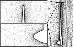
Fig. 1. Unstructured mesh construction of rotating parts on normal cut plane
5. Grid Study
Table 1. Variation of ![]() versus number of mesh elements for case 7
versus number of mesh elements for case 7
| Number of elements | about rotor axis |
| 649,358 | 0.05767 |
| 1,203,423 | 0.05753 |
| 1,923,117 | 0.05747 |
| 2,602,863 | 0.05745 |
| 3,489,261 | 0.05743 |
Obviously, no numerical simulation is reliable without a grid study. The first rough mesh, generated at the first step often contains cells especially near wall or in boundary layer region, which is not capable of capturing all gradients effects or phenomena happening in separation region. So by slightly changing the mesh, the results may take new values. Therefore, the mesh must be treated in a couple of steps to get results, which become independent of mesh size. The first mesh generated in this study contains around 650,000 cells, more of which are in cylindrical sliding region. Then, the mesh was treated in five stages leading the mesh size to reach 3,500,000 cells. During five level of treatment it was seen that the results don’t change considerably, which shows independency is already achieved. Consequently, the first grid was chosen because of simplicity in computational cost. Table 1 shows the details about number of elements and variation of moment coefficient (![]() ) during grid study process for case 7, RNG method (as a sample case). It must be mentioned that solution residuals values in whole domain were chosen as the convergence criteria in order to make sure that solution is converged all across the domain. This was evaluated by checking residual contours.
) during grid study process for case 7, RNG method (as a sample case). It must be mentioned that solution residuals values in whole domain were chosen as the convergence criteria in order to make sure that solution is converged all across the domain. This was evaluated by checking residual contours.
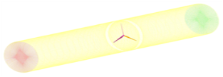
Fig. 2. Fluid domain for CFD model, including rotating unstructured and stationary structured parts
6. Turbulent Model Investigation
Referring to brochure data given in [17], the cut-in and cut-off speeds for Vestas V80 HAWT are respectively 4 m/s and 25 m/s. Taking these two values as minimum and maximum of free stream velocity range, minimum and maximum values of Reynolds number can be calculated, based on blade length, as 1.1e+7 and 6.7e+7. Even the minimum value is higher than critical Reynolds number for transition to outer turbulent flow. Hence, one can assume the flow fully turbulent. Thanks to ![]() RNG and
RNG and ![]() SST methodologies for both near-wall and far distance regions, surely all turbulent and boundary layer phenomena, including separation, viscous layer interactions and wakes are investigated in the simulations, using these models. To get results for a wide performance range of turbine, 22 cases were considered, the variant parameters of which are free stream velocity and mean pitch angle of blades.
SST methodologies for both near-wall and far distance regions, surely all turbulent and boundary layer phenomena, including separation, viscous layer interactions and wakes are investigated in the simulations, using these models. To get results for a wide performance range of turbine, 22 cases were considered, the variant parameters of which are free stream velocity and mean pitch angle of blades.
7. Wall y+ Number
To fully capture the fluid flow behaviour in boundary layer region, we need to correctly set![]() distance as the first cell height. According to a correlation for
distance as the first cell height. According to a correlation for ![]() valuewe have the following equation for our cell-based method:
valuewe have the following equation for our cell-based method:
![]() (17)
(17)
where![]() is the dimensionless distance from the wall. As mentioned before, the Reynolds number is around 6.7e+7. Therefore, having above equation and taking
is the dimensionless distance from the wall. As mentioned before, the Reynolds number is around 6.7e+7. Therefore, having above equation and taking ![]() as 30,
as 30,![]() becomes about 0.0026 m (2.6 mm). Setting this value in mesh generation, we can make sure all interactions in the boundary layer are fully captured.
becomes about 0.0026 m (2.6 mm). Setting this value in mesh generation, we can make sure all interactions in the boundary layer are fully captured.
8. Output Power Calculation
To calculate the output power of the turbine, moment coefficient value should be used. Having angular velocity and moment about rotating axis of turbine power delivered by turbine can be defined. The torque T can be calculated by the following equation:
![]() (18)
(18)
where![]() and
and ![]() are density and velocity of free stream, respectively,
are density and velocity of free stream, respectively,![]() (moment coefficient) is obtained directly through developed CFD code,
(moment coefficient) is obtained directly through developed CFD code, ![]() is circle area swept by rotating bladesand R is blade radius in SI units. Assuming standard condition the value of 1.225
is circle area swept by rotating bladesand R is blade radius in SI units. Assuming standard condition the value of 1.225 ![]() is used for air density. Other parameters, provided by the manufacturer [17], are given in table 2.
is used for air density. Other parameters, provided by the manufacturer [17], are given in table 2.
Table 2. Brochure data for Vestas V80 [17]
| Power Regulation | Pitch regulated with variable speed |
| Rated power | 2000 kW |
| Cut-in wind speed | 4 m/s |
| Rated wind speed | 16 m/s |
| Cut-out wind speed | 25 m/s |
| Rotor diameter | 80 m |
| Swept area | 5027 m2 |
| Blade length | 39 m |
One important characteristic of any wind turbine is the tip speed ratio, ![]() , which means at what wind speed, turbine will rotate at specific angular velocity. It is defined by following equation:
, which means at what wind speed, turbine will rotate at specific angular velocity. It is defined by following equation:
![]() (19)
(19)
where R is blade radius and ![]() is turbine angular velocity in SI units. Tip speed ratio values applied in this study are calculated from angular velocity plot given by [18]. The corresponding curve is given in Fig. 3. Taking account these values in our calculations, data set in approach are given in table 3.The most important factor used to evaluate overall performance of a wind turbine is its power coefficient, which is defined as:
is turbine angular velocity in SI units. Tip speed ratio values applied in this study are calculated from angular velocity plot given by [18]. The corresponding curve is given in Fig. 3. Taking account these values in our calculations, data set in approach are given in table 3.The most important factor used to evaluate overall performance of a wind turbine is its power coefficient, which is defined as:
![]() (20)
(20)
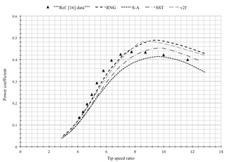
Fig. 3. Rotor speed and pitch angle both as a function of wind speed [18]
9. Results and Discussion
The corresponding results for four mentioned CFD methods are given in Fig.4. Clearly the ![]() RNG has given bigger moment coefficient and output power values for all free stream velocities. So did the
RNG has given bigger moment coefficient and output power values for all free stream velocities. So did the ![]() method, but with less deviation from manufacturer’s brochure data, while
method, but with less deviation from manufacturer’s brochure data, while ![]() SSTand Spalart-Allmaras models have under-predicted the power output values after around infinity velocity of 7m/s. It is to be noted that the wind turbine geometry simulated in this study is not the same as experimented by the manufacturer; mainly because of three reasons: (1) the Vestas V80 turbine geometry used here doesn’t include its nacelle and tower, so the their effect on the air flow is neglected; (2) These turbines are mounted at hub height of around 70-80 m above the ground[18], while we have assumed the rotating blades free in the air, so this height is not considered in the simulations; (3) wind turbines are usually installed together in farms in big quantities resulting in reduction of overall performance of turbines, mainly because of wakes produced by adjacent turbines. But current study doesn’t take this issue in to account, so that the results are optimistic to some extent.
SSTand Spalart-Allmaras models have under-predicted the power output values after around infinity velocity of 7m/s. It is to be noted that the wind turbine geometry simulated in this study is not the same as experimented by the manufacturer; mainly because of three reasons: (1) the Vestas V80 turbine geometry used here doesn’t include its nacelle and tower, so the their effect on the air flow is neglected; (2) These turbines are mounted at hub height of around 70-80 m above the ground[18], while we have assumed the rotating blades free in the air, so this height is not considered in the simulations; (3) wind turbines are usually installed together in farms in big quantities resulting in reduction of overall performance of turbines, mainly because of wakes produced by adjacent turbines. But current study doesn’t take this issue in to account, so that the results are optimistic to some extent.
Therefore considering above assumptions, roughly we can expect that the results should show some over prediction of power values. The ![]() RNG has over-predicted values with about 22~50% deviation, least of which corresponds to rated power of turbine, while maximum error is for cut-in velocities of turbine. However,
RNG has over-predicted values with about 22~50% deviation, least of which corresponds to rated power of turbine, while maximum error is for cut-in velocities of turbine. However, ![]() results show smaller deviation and can be labelled as more "realistic" model among the other approaches regarding assumptions of the problem.
results show smaller deviation and can be labelled as more "realistic" model among the other approaches regarding assumptions of the problem.
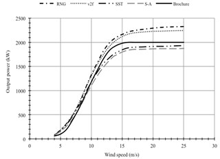
Fig. 4. Power curves of four used CFD methods compared with brochure data
In addition to power curve (![]() diagram), another important plot, which is never disregarded by wind turbine designers, is the variation of power coefficient with tip speed ratio; because we are always looking for a quasi-constant
diagram), another important plot, which is never disregarded by wind turbine designers, is the variation of power coefficient with tip speed ratio; because we are always looking for a quasi-constant![]() values over various operating wind velocities[19]. The corresponding plots extracted from simulation results are given in Fig.5 as well as data obtained in [19]. As indicated in Fig.5, the peak value of pressure coefficient (0.452) is well predicted by
values over various operating wind velocities[19]. The corresponding plots extracted from simulation results are given in Fig.5 as well as data obtained in [19]. As indicated in Fig.5, the peak value of pressure coefficient (0.452) is well predicted by ![]() SST model in comparison with that of experiments, which is about 0.436. This could be because of the model’s intrinsic assumption, that is, the hybrid shear stress transport model solves simplified Navier-Stokes equations for low Reynolds regime near the wall, while it uses high Reynolds assumption for region outside the boundary layer.
SST model in comparison with that of experiments, which is about 0.436. This could be because of the model’s intrinsic assumption, that is, the hybrid shear stress transport model solves simplified Navier-Stokes equations for low Reynolds regime near the wall, while it uses high Reynolds assumption for region outside the boundary layer.
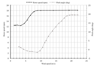
Fig. 5. Power coefficient versus tip speed ratio plot of four used CFD models and trend given in [17]
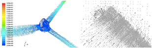
Fig. 6. (a) Pathlines by velocity magnitude and (b) velocity vectors showing mild separation around blade tip
Given the path lines, determined by velocity magnitude, and velocity vectors obviously showing mild separation around blade tip in Fig. 6, as a future work it may be useful to mount winglet-like end plates on blade tips to prevent separation. By employing such plates, clearly the flow would pass the tip area smoother, hence with fewer disturbances.
The pressure coefficient distribution on the surface and leading edge of the wind turbine’s blades is illustrated in Fig.7. As indicated, the pressure coefficient values increase on the blade as nearing to the leading edge. This is due to stagnation near the leading edge; the fluid particles almost stop when they meet the first contact area on blades, which means a sudden fall in velocity magnitude. The change in pressure is accounted for by the Bernoulli equation, which means for horizontal fluid flow, a decrease in the velocity of flow will result in an increase in static pressure. This fact could be help to designers to consider such a magnificent load on the leading edge to prevent destructive phenomena such as fatigue or creeping in a more effective way.
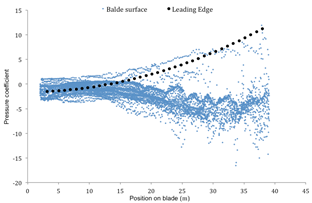
Fig. 7. Pressure coefficient distribution along blade surface and the leading edge
Finally, as discussed earlier, the closest results for generated output power, in comparison with the experiments, are related to k-epsilon RNG turbulence method. However, for the power coefficient all employed methods have given acceptable outcomes for output power.
Table 3. Cases with associated data and results
| Case | (m/s) | (rad/s) | Pitch angle (deg) | k-w SST | k-e RNG | S-A | v2-f | |
| 1 | 4 | 1.319 | 12.865 | -1.75 | 78.5 | 84.9 | 67.7 | 83.6 |
| 2 | 5 | 1.299 | 10.128 | -1 | 188.4 | 215.1 | 151 | 167.2 |
| 3 | 6 | 1.361 | 8.849 | 0 | 291.2 | 336.6 | 261.3 | 318.8 |
| 4 | 7 | 1.508 | 8.402 | 0.8 | 491.1 | 499.2 | 304.1 | 512.2 |
| 5 | 8 | 1.676 | 8.168 | 1 | 697.9 | 722.8 | 652.4 | 747.4 |
| 6 | 9 | 1.843 | 7.987 | 1.25 | 935.5 | 1000.3 | 917.7 | 1063.6 |
| 7 | 10 | 1.885 | 7.351 | 1.75 | 1158.6 | 1338.8 | 1096.3 | 1306.6 |
| 8 | 11 | 1.885 | 6.683 | -0.5 | 1408.2 | 1626.2 | 1306.6 | 1549.6 |
| 9 | 12 | 1.885 | 6.126 | -3 | 1561.3 | 1827.3 | 1483.5 | 1803.1 |
| 10 | 13 | 1.885 | 5.655 | -6.5 | 1704.7 | 2003.1 | 1643.2 | 1931.2 |
| 11 | 14 | 1.885 | 5.251 | -10.5 | 1813.8 | 2095.4 | 1737.8 | 2040.9 |
| 12 | 15 | 1.885 | 4.901 | -12 | 1853.2 | 2078.6 | 1795.3 | 2137.6 |
| 13 | 16 | 1.885 | 4.595 | -13.75 | 1882.9 | 2218.6 | 1837.1 | 2164.2 |
| 14 | 17 | 1.885 | 4.324 | -15.8 | 1898.3 | 2246.5 | 1852.8 | 2192.5 |
| 15 | 18 | 1.885 | 4.084 | -17.5 | 1900.2 | 2255.7 | 1853.4 | 2216 |
| 16 | 19 | 1.885 | 3.869 | -18.75 | 1909.4 | 2278.9 | 1860.8 | 2229.1 |
| 17 | 20 | 1.885 | 3.676 | -19 | 1912.8 | 2293.5 | 1867.4 | 2231.7 |
| 18 | 21 | 1.885 | 3.501 | -19 | 1917 | 2302.7 | 1866 | 2236.9 |
| 19 | 22 | 1.885 | 3.342 | -19 | 1917.6 | 2318.3 | 1868.5 | 2238.4 |
| 20 | 23 | 1.885 | 3.196 | -19 | 1921.3 | 2319.4 | 1868.7 | 2239.5 |
| 21 | 24 | 1.885 | 3.063 | -19 | 1928.5 | 2324.5 | 1869.8 | 2242.2 |
| 22 | 25 | 1.885 | 2.941 | -19 | 1932.7 | 2326.6 | 1873.7 | 2244.7 |
10. Conclusion
The main objective of this study was to numerically investigate the turbulent airflow passed a commercial horizontal axis wind turbine using four different turbulence models with least simplifying considerations to get the most possible precise results, and then comparing gained results with those of experimental methods as well as brochure data provided by the manufacturer. The significant outstanding difference between current study and the others is inclusion of boundary layer and near-wall effects in the simulations, which gives more realistic and accurate results. It was demonstrated that results of performed simulations were in good agreement with experimental data presented previously. The closest results, for generated output power, compared to experiments are associated with the k-epsilon RNG turbulence method. In addition, due to the mild separation occurring at the blades tips, it is suggested to mount winglet-like end plates to reduce the induced drag and improve the overall performance of the turbine.
References
- Widjanarko SM. Steady Blade Element Momentum Code for wind turbine design validation tool. Internship – Vestas Wind System A/S, Twente University, 2010.
- Hartwagner D, Horvat A. 3D Modelling of a Wind Turbine Using CFD.NAFEMS Conference, 2008.
- Galdamez RG, Ferguson DM, Gutierrez J.R. Design Optimization of Winglets for Wind Turbine Rotor Blades Report. B.S. thesis, Florida International University, 2011.
- Tahani M, Sokhansefat T, Rahmani K, Ahmadi P. Aerodynamic Optimal Design of Wind Turbine Blades using Genetic Algorithm. Energy Equipment and Systems, 2014; 2(2):185-193.
- Tangler J. The Nebulous Art of Using Wind-Tunnel Airfoil Data for Predicting Rotor Performance. NREL/CP-500-31243, National Renewable Energy Laboratory, Colorado, 2002.
- A. Sedaghat, M. Mirhosseini.Aerodynamic design of a 300 kW horizontal axis wind turbine for province of Semnan. Energy conversion and management. 2012; 63:87-94.
- Sezer-Uzol N, Long LN.3-D Time-Accurate CFD Simulations of Wind Turbine Rotor Flow Fields. AIAA paper No.2006-0394, 2006.
- Zhou B, Chow FK. Turbulence Modeling for the Stable Atmospheric Boundary Layer and Implications for Wind Energy. Flow, Turbulence and Combustion, 2012;88:255–277.
- ChathelainP, Backaert S, Winkelmans G, Kern S.Large Eddy Simulation of Wind Turbine Wakes, Flow, Turbulence and Combustion, 2013;91:587–605.
- Jeon M, Lee S, Lee S. Unsteady aerodynamics of offshore floating wind turbines in platform pitching motion using vortex lattice method, Renewable Energy, 2013, p.207–212.
- Lanzafame R, Mauro S, Messina M. Wind turbine CFD modeling using a correlation-based transitional model, Renewable Energy, 2013; 52: 31-39.
- Mohamed A. Sayed, Hamdy A. Kandil, Ahmed Shaltot. Aerodynamic analysis of different wind-turbine blade profiles using finite-volume method.Energy conversion and management.2012; 64:541-550.
- Yakhot V, Orszag SA. Renormalization Group Analysis of Turbulence: I. Basic Theory. Journal of Scientific Computing, 1986; 1(1):1-51.
- Menter FR. Two-Equation Eddy-Viscosity Turbulence Models for Engineering Applications. AIAA Journal, 1994; 32(8):1598-1605.
- Laurence DR, Uribe JC, Utyuzhnikov SV. A Robust Formulation of the v2-f Model. Flow, Turbulence and Combustion, Kluwer Academic Publishers, 2004;73: 169–185.
- Durbin PA, Pettersson Reif BA. Statistical Theory and Modeling for Turbulent Flows.Wiley, Chichester, UK; 2001.
- HansenKS, BarthelmieRJ, JensenLE, Sommer A. The Impact of Turbulence Intensity and Atmospheric Stability on Power Deficits Due to Wind Turbine Wakes at Horns Rev Wind Farm. Wind Energy, 2012; 15: 183–196. doi: 10.1002/we.512.
- www.vestas.com
- Wood D. Small Wind Turbines, Analysis, Design, and Application. Springer; 2011.


