
American Journal of Renewable and Sustainable Energy, Vol. 1, No. 1, May 2015 Publish Date: Apr. 10, 2015 Pages: 1-8
An Optimal Feed-In-Tariff Policy for Renewable Energies Using A Markov Model
Shahab Bahrami*, Aras Sheikhi
Department of Electrical Engineering,Sharif University of Technology, Tehran, Iran
Abstract
Recent developments in renewable energy generation make it possible for renewable sectors to supply considerable share of electricity all around the world. As these sectors get larger, more attention is paid to the implementation of supportive strategies with the aim of motivating renewable energy (RE) developers. At present, Feed-In-Tariff (FIT) policies are regarded as one of the efficient strategies in stimulating renewable energy development and as such, designing approaches and controlling options of these policies are of utmost important. This paper presents a method based on a Markov chain model to investigate the economic benefits associated with the FIT policies. The proposed technique is used to study different aspects of FIT policies by dividing electricity prices, generation conditions and developer's cost-benefits into distinct states. Simulations are performed on a sample wind turbineto examine various features of designing premium price FIT policy.
Keywords
Feed-In-Tariff, Markov Chain Model, Premium Price FIT, Renewable Energy
Received: March 23, 2015
Accepted: April 5, 2015
Published online: April 10, 2015
@ 2015 The Authors. Published by American Institute of Science. This Open Access article is under the CC BY-NC license. http://creativecommons.org/licenses/by-nc/4.0/
1. Introduction
Renewable energy technologies (RET) play a significant role in electricity generation; andthus, more efforts are made to expand these eco-friendly energies [1]. The reasons for supporting RET vary from one country to another and are strongly dependent on the overall situation from the environmental phases to the economic and social aspects. Commonly, the main reasons for supporting renewable energies (RE) are the global warming, fuel depletion, security of supply, expansion of distributed generations (DGs) [2], and expansion of plug-in hybrid vehicles [3].
Experiences around the world have shown that the strategies devised to support RE developers play an undeniable role in developing RETs [4].Based on such experiences, various schemes have been developed and successfully implementedto reassure the RE sectors, such as Renewable Obligation Certificate (ROC) [5], Non-Fossil Fuels Obligation (NFFO) [6], Renewable Energy Certificates (REC) [7], and Feed-In-Tariffs (FIT) [8].
Among the above policies, FIT is known as the one of the successful strategies [9]. FIT refers to an above market energy payment for the electricity fed into power grid generated bya renewable energyresource.Under this strategy, the government guarantees to purchase all the electricity generated by renewable generations according to a certain remuneration model [9], [10].
FIT policies are categorized into two main groups as shown in Fig. 1: market independent (fixed price) policy and market dependent (premium price) policy.[11]. As shown in this figure, in the market independent FIT, the producersells electricity on higher rate (solid line) as comparedwith the market price(dashed line) in the initial years of the project as an incentive.This rate is fixed through the project period.However, the market pricemay increase annually and after a few years, the producer may receive less as comparedwith the market price. On account of this fact, the RE developer is motivated to expand its facilities andgenerate as much electricity as possible in the initial years of the project [11].
In themarket dependent FIT policy,the RE developerreceivesacertain premium on top of the marketprice as an incentive for the whole duration of the project period.However,the developer might face more difficulties in the beginning of the project as comparedwith the fixed price policysince less incentive is given to the RE developer [11].In both policy models, incentive payments are determined with respect to some critical parameters such as the technology aspects (type, maturity, generation cost, etc.), the environmental conditions (wind speed, sunshine radiation), the project size, the plant sites and the electricity application (base or peak load) [12]. Details of the differences between these two types of policies are discussed in [13]. Policy makers analyze several designing factors in order to employ the mentioned policies [12]. Not only do they need accurate information about current and near-future markets, but also they must be able to accurately predict the long-term market and technological trends [13]. A number of approaches have been proposed to analyze FIT models. Muhammad-Sukki in [14] have studied general financial aspects of FIT in Malaysia and compared the results with the other countries. Dusonchet and Telaretti [15] have investigated different incentive policies in Western European countries and performed economic analyses on various aspects of these policies. Lesser and Su [16] have overviewed the performance of some current FIT policies in different countries and modeled a two-part FIT on a forward capacity market to ensure security of development and stability of the whole market. Shrimali and Baker [17] have derived an optimal FIT schedule under production-based learning. They have performed two dynamic approaches, the learning–by-doing (LBD) and the economies of scale (EOS) method to investigate how the levelized cost of renewable technologies can be reduced.
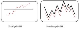
Figure 1. Market dependent and independent FIT Policies(the dashed line is the market price and the solid line is the FIT price [11].
In [18], the impact of regulatory uncertainty induced by regulators considering moves from a FIT scheme to a moremarket-oriented regulatory regime is studied. Besides, numerical solutions reflecting current and expected future revisions in FIT levels is developed to show the potential changes in regulatory regimes. In [19], different FIT policies is studied for Photovoltaic systems. The advantages and disadvantages of each policy is investigated and compared. Lack of a comprehensive method with practical characteristics is discernible. This paper presents a novel approach, based on the Markov chain theoryto analyze various scenarios of the FIT policies by modelingthe cost and benefit of the RE developer during the project period. Furthermore, a sensitivity analysis is performed to investigate the impacts of variation in the parameters in the FIT model.
2. Price andFIT models
Markov chain is a mathematical model that undergoes transitions from one state to another (from a finite or countable number of possible states in a system) in a chainlike manner [20]. It is a random process characterized as memory less (i.e. exhibiting the Markov property), which means that the next state depends only on the current state and not on the entire past. Markov chains have many applications as statistical models of the real-world processes, and can be used for modeling the systems with random behavior. Under this model, the system behavior is described by different states .
There are two main Markov models: the discrete model and continuous model [21].The continuous one is utilized in this paper to model the electricity price, generation, load demand, and cost-benefit of RE developer. In all steps, the Markov chain theory will be applied to calculate the main parameters such as the state probabilities and the transition rates. The explanation of this theory is beyond the scope of this paper and is presented in detail in [21]-[24].
2.1. Price Model
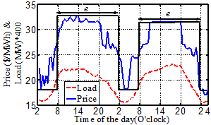
Figure 2. Daily electricity price and load variation in NSW region inAustralia.(Source: AEMO [25])
Since the electricity price is a reflection of the electricity loadvariation, the price can be determined as a stochastic system in time, which can be modeled with Markov chains [23].Fig. 2 shows the electricity price and the load demand variation in a typical dayin the NSW region in Australia [25].J.D. Hall et al [23]have described how the load demand can be represented by a simple Markov chain model regarding to peak levels. Since the electricity price almost always follows the load demand in competitive markets, it can be modeled similarly. Consequently, the price variation can be approximated by two step function as a daily price model. This model consists of a peak price level with duration ![]() (exposure factor), and a low price with duration of
(exposure factor), and a low price with duration of![]() for the remaining time. This two-level daily model for the electricity price can be used in all days of period
for the remaining time. This two-level daily model for the electricity price can be used in all days of period![]() . Fig. 3 represents an approximation model for the price cycle for period
. Fig. 3 represents an approximation model for the price cycle for period![]() days. To obtain the Markov model of electricity price, it is assumed that the price data for the pastyears (e.g., the past 10 years) are available. First, the price data of each of the previous years are discounted back to its value in the first year using the average inflation rate. Second, the calculated values are considered to determine a two-level model for the electricity price in upcoming years.
days. To obtain the Markov model of electricity price, it is assumed that the price data for the pastyears (e.g., the past 10 years) are available. First, the price data of each of the previous years are discounted back to its value in the first year using the average inflation rate. Second, the calculated values are considered to determine a two-level model for the electricity price in upcoming years.
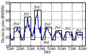
Figure 3. Price cycle approximation with peak levels and fixed low level.(Source: AEMO [25])
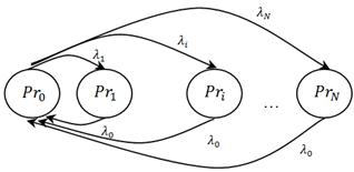
Figure 4. Markov model for the electricity price.
The Markov chain for this price model is depicted in Fig. 4. This model contains ![]() states
states![]() ,
,![]() ,…,
,…,![]() andeach state occurs on average
andeach state occurs on average ![]() times during the pastyears [23].The peak price returns to the low level (usually during nights) every day [23]. Additionally, the exposure factors for all days can beassumed tobe equal to the average of exposure factors for all days [25]. These assumptions are acceptable for modeling the market price in a period of a month or a year. To study longer cycles, the price levels for the initial year should be updated by taking into account the inflation rate.Therefore, the proposed model can be applied with new parameters [23], [24].
times during the pastyears [23].The peak price returns to the low level (usually during nights) every day [23]. Additionally, the exposure factors for all days can beassumed tobe equal to the average of exposure factors for all days [25]. These assumptions are acceptable for modeling the market price in a period of a month or a year. To study longer cycles, the price levels for the initial year should be updated by taking into account the inflation rate.Therefore, the proposed model can be applied with new parameters [23], [24].
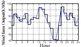
Figure 5. Two states Markov model for Generation and load for certain day. (Source: AEMO [25])
2.2. Generation-Load State Model
On a given day, output generation of a RE plant varies hourly and may be different from its local load demand. As an example, Fig. 5 shows the output power for a certain wind turbine in Tasmania[26].Using the Markov chain theory [20], generation of the RE plant, as shown in Fig. 5, can be approximately modeled by a number ofaveragestates denoted by![]() in descending order of generation level. In this paper, for the sake of simplicity, it is assumed that the load is constant. The method canbealso applied for variable load demand which can be modeled with different states (see the general case in [21] and [22]).By combining thegeneration and loadMarkov models, margin states are defined as the difference between the available capacity and the load demand [21]. They are represented by
in descending order of generation level. In this paper, for the sake of simplicity, it is assumed that the load is constant. The method canbealso applied for variable load demand which can be modeled with different states (see the general case in [21] and [22]).By combining thegeneration and loadMarkov models, margin states are defined as the difference between the available capacity and the load demand [21]. They are represented by ![]() states
states![]() as follows:
as follows:
![]() (1)
(1)
![]() (2)
(2)
Index ![]() denotes the last state in which generation is more than load.Note that with generation states ordered descending,
denotes the last state in which generation is more than load.Note that with generation states ordered descending, ![]() values are also in descending order.The state probabilities and transition rates ofthe margin states can be calculated using the Markov chain theories which are explained in detail in [21]. For simplicity and without loss of generality, it is considered that there are m distinct generation states all equally likely. Thus, the transition rate and probability of each state are
values are also in descending order.The state probabilities and transition rates ofthe margin states can be calculated using the Markov chain theories which are explained in detail in [21]. For simplicity and without loss of generality, it is considered that there are m distinct generation states all equally likely. Thus, the transition rate and probability of each state are
![]() (3)
(3)
![]() (4)
(4)
An advantage of modeling the generation and load using the Markov theory is the ability of modeling variation in the renewable energy sources such as wind turbines and PV cells [22]. Moreover, by considering more levels in shorter time intervals and acquiringmore data on the past behavior of the generated power, more accurate margin states model can be obtained [23].
2.3. Cost-Benefit State Model
To analyze FIT policies usingMarkov model, it is required to develop a cost-benefit Markov model that shows the costs and benefits of trading electricity between the market and the RE developer. In steps ![]() and
and![]() , twoMarkov chain models are obtained, one for the market price levels and the other one for the margin levels. It can be considered that for the small scale of renewable generations in the electricity markets, these two models are mutually exclusive. The combination of these two state models will be a Markov model with
, twoMarkov chain models are obtained, one for the market price levels and the other one for the margin levels. It can be considered that for the small scale of renewable generations in the electricity markets, these two models are mutually exclusive. The combination of these two state models will be a Markov model with ![]() states.In this mixed Markov model, state
states.In this mixed Markov model, state ![]() (
(![]() denotes the state, in which the margin level is in state
denotes the state, in which the margin level is in state ![]() and the market price is in state
and the market price is in state![]() .Method of combination the twoMarkov models is similar to the method used in developing margin states model from the load and capacity, as discussed in [21].
.Method of combination the twoMarkov models is similar to the method used in developing margin states model from the load and capacity, as discussed in [21].
To obtain a Markov model for the cost and benefit of developer in the premium price FIT scheme, it is essential to distinguish all situations in which the RE developer would make benefit or pay cost. In this paper, it is assumed that the FIT payment is"Net",which means that the RE units sell their extra generation over the local load to the grid and receive FITsupport [13]. This approach is different from "Gross" payment, in which the RE units receive government's support for all their generated electricity [13]. Accordingly, positive margin state![]() , corresponds to the states
, corresponds to the states![]() (0
(0![]() ), in which the developer would sell its extra generated electricity (with the amount of
), in which the developer would sell its extra generated electricity (with the amount of ![]() to the grid based on FIT price and makes benefit.On the contrary, if the load demand exceeds the generation of RE plant then the developer will buy electricity from the grid but based on the market price. In this case, we are in the margin state
to the grid based on FIT price and makes benefit.On the contrary, if the load demand exceeds the generation of RE plant then the developer will buy electricity from the grid but based on the market price. In this case, we are in the margin state ![]() corresponds to the states
corresponds to the states![]() (0
(0![]() ).It is important to note that the Gross FIT policies can also be examined with a little change in modeling of the cost and benefit. In addition to the above issues, there are other costs such as investment, operation and maintenance costs that will be considered in the model in the simulation.Consistent with themarket dependent FIT policies, the premium amount declines asthe electricity prices increase [13]. In its simplest form, when the current electricity price is in the lower levels (first
).It is important to note that the Gross FIT policies can also be examined with a little change in modeling of the cost and benefit. In addition to the above issues, there are other costs such as investment, operation and maintenance costs that will be considered in the model in the simulation.Consistent with themarket dependent FIT policies, the premium amount declines asthe electricity prices increase [13]. In its simplest form, when the current electricity price is in the lower levels (first ![]() levels), the developer sells its extra generation at
levels), the developer sells its extra generation at![]() percenthigher than the market electricity price.Ifthe current market price beat the higher levels,the developer will sell its extra generation at "
percenthigher than the market electricity price.Ifthe current market price beat the higher levels,the developer will sell its extra generation at "![]() " percent higher than the market price, and
" percent higher than the market price, and![]() . Parameters
. Parameters ![]() and
and ![]() are premiums of the market dependent FIT. This kind of FIT modeling mainly prevents windfalls phenomena that cause unreasonable profits for the RE developers [13]. Accordingly,the cost and benefit for premium priceFITare as follows:
are premiums of the market dependent FIT. This kind of FIT modeling mainly prevents windfalls phenomena that cause unreasonable profits for the RE developers [13]. Accordingly,the cost and benefit for premium priceFITare as follows:
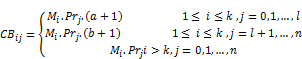 (5)
(5)
where![]() ($/year) denotes the state
($/year) denotes the state ![]() of the cost-benefit model.This approach can also be applied for modeling other types of FIT policies. Additionally, the above model contains only the cost and benefit of buying and selling electricity; however,other costs such as the investment,operation and maintenance costscan be added to the model to determinethe total RE developer's profit.
of the cost-benefit model.This approach can also be applied for modeling other types of FIT policies. Additionally, the above model contains only the cost and benefit of buying and selling electricity; however,other costs such as the investment,operation and maintenance costscan be added to the model to determinethe total RE developer's profit.
3. A Premium Price Fit
In this section,the proposedmodel is used for a specific wind turbine project, to investigate the characteristics of a given FIT policy. The results are used to present design issues for an appropriate premium price FIT.The price levels and transition rates are given in Table I. The operational data of the wind turbine is given in Table II.To obtain theMarkov model for the electricity market, it is assumed that the simulation is performed for the NSW marketfrom 2006 to2014 [25]. The Markov model is obtained for the next 30 years of the project period. The parameters of this model areD=365(days),![]() ,
,![]() . Hence,nine peak levels and one low level for the price in each year is considered.According to Table I, the data for this price model can be calculated asshown in Table III. The generated electricity is also modeled with
. Hence,nine peak levels and one low level for the price in each year is considered.According to Table I, the data for this price model can be calculated asshown in Table III. The generated electricity is also modeled with![]() distinctequally likely levels with transition rates of
distinctequally likely levels with transition rates of ![]() (trans/hour) = 24(trans/day). Local load level isassumed to be constant at
(trans/hour) = 24(trans/day). Local load level isassumed to be constant at![]() .Accordingly, themargin states model data for this proposed turbine are calculated as shownin TableIV.Using the data given in Table IV for the wind turbine, the present worth of total cost for studied turbine can be calculated as:
.Accordingly, themargin states model data for this proposed turbine are calculated as shownin TableIV.Using the data given in Table IV for the wind turbine, the present worth of total cost for studied turbine can be calculated as:
![]() 233,600($) (6)
233,600($) (6)
where![]() isthe generation capacity of the wind turbine.
isthe generation capacity of the wind turbine.![]() is the investment cost.
is the investment cost.![]() is the operation and maintenance cost.
is the operation and maintenance cost.![]() is the Inflation rate.Renewable sources have high capital cost.Hence, it is imperative for the RE developer to setup a project with an acceptablepayback period. In the following subsection, the effects of FIT parameters will be examined to design the best policy.
is the Inflation rate.Renewable sources have high capital cost.Hence, it is imperative for the RE developer to setup a project with an acceptablepayback period. In the following subsection, the effects of FIT parameters will be examined to design the best policy.
Table I. Transition rates and state probability for price Markov model
| State number | Price States Data | |
| Transition rate to the state | State probability | |
| Low level |
|
|
| Peak level |
|
|
Table II. Operational data for the proposed wind turbine
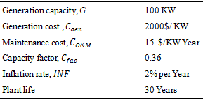
Table III. Price levels, transition rates and probability of each price level
| Price level state | Price level data | |||
| Price level |
|
|
| |
| 1 | 37 | 73 | 0.4 | 0.100 |
| 2 | 39 | 63 | 0.34 | 0.085 |
| 3 | 41 | 51 | 0.28 | 0.070 |
| 4 | 43 | 44 | 0.24 | 0.060 |
| 5 | 45 | 37 | 0.20 | 0.050 |
| 6 | 47 | 32 | 0.18 | 0.045 |
| 7 | 49 | 32 | 0.18 | 0.045 |
| 8 | 51 | 25 | 0.14 | 0.035 |
| 9 | 53 | 8 | 0.04 | 0.010 |
| 0 | 35 | 365 | 2.0 | 0.500 |
Table IV. Generation and margin levels for a sample wind turbine
| State number | Generation levels data | |||
| Generation level | Margin level |
|
| |
| 1 | 72 | 62 | 24 | 0.166 |
| 2 | 64 | 54 | 24 | 0.166 |
| 3 | 56 | 46 | 24 | 0.166 |
| 4 | 48 | 38 | 24 | 0.166 |
| 5 | 40 | 30 | 24 | 0.166 |
| 6 | 32 | 22 | 24 | 0.166 |
| 7 | 24 | 14 | 24 | 0.166 |
| 8 | 16 | 6 | 24 | 0.166 |
| 9 | 8 | -3 | 24 | 0.166 |
| 10 | 0 | -10 | 24 | 0.166 |
3.1. Premium FIT calculation
Fig. 6 showsthe payback period of implementing the proposed wind turbine in terms of FIT payment parameter![]() . It is assumed that
. It is assumed that![]() is applied to the three highest price levels. By increasing the payment, the payback period will decrease, but choosing a proper payment depends on various factors from both RE developers' and thegovernment's points of view. For instance, choosing
is applied to the three highest price levels. By increasing the payment, the payback period will decrease, but choosing a proper payment depends on various factors from both RE developers' and thegovernment's points of view. For instance, choosing![]() %, results in about 20years payback period. Besides, Fig. 7 illustrates that by choosing
%, results in about 20years payback period. Besides, Fig. 7 illustrates that by choosing![]() = 53% as an incentive, the RE developer's present value of gross benefit in 30 years will be 8.5
= 53% as an incentive, the RE developer's present value of gross benefit in 30 years will be 8.5![]() ($), which is enough for such a small-scaled project.The results presented indicate that the proposed method can easily model the cost, benefit and payback period of the RE developer to design a proper FIT policy.
($), which is enough for such a small-scaled project.The results presented indicate that the proposed method can easily model the cost, benefit and payback period of the RE developer to design a proper FIT policy.
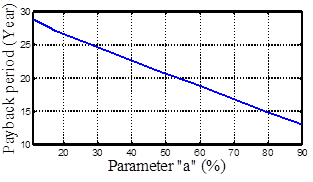
Figure 6. Payback period in terms of incentive payment.

Figure 7. Total gross benefit in terms of parameter"a".
3.2. Windfall Profit
Unreasonable values for FIT parameters could resultin more than necessary profit or windfall profit for the RE developer [13]. A windfall profitrefers toan unreasonable high profits caused by rising market price unexpectedly. In case of premium price FIT policy, the improper value of parameter ![]() may result in windfall profit for the RE developers [13]. Fig. 8 depicts the impact of increasing premiums in lower and higher price levels. It can be seen that for a given year, an increase in parameter b from 10% to 100%results in less increase in the benefit than that of increasing parameter a from 30% to 60%. This indicates that increasing premiums for lower levels result in much more benefit for the RE developers. This fact implies that high premiums in higher price levels result in not only inflation and windfall profit which are not acceptable in the market, but also a slight increase in the developer's benefit inlong-term. Accordingly, to avoid these consequences, policy makers lmost always choose low payment in higher market price [13].
may result in windfall profit for the RE developers [13]. Fig. 8 depicts the impact of increasing premiums in lower and higher price levels. It can be seen that for a given year, an increase in parameter b from 10% to 100%results in less increase in the benefit than that of increasing parameter a from 30% to 60%. This indicates that increasing premiums for lower levels result in much more benefit for the RE developers. This fact implies that high premiums in higher price levels result in not only inflation and windfall profit which are not acceptable in the market, but also a slight increase in the developer's benefit inlong-term. Accordingly, to avoid these consequences, policy makers lmost always choose low payment in higher market price [13].
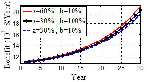
Figure 8. Impact of increasing parameter "b" and parameter "a" on benefit.
3.3. Gradual Degression of RE Premium
FITs often include technology improvement factors designed to reduce payments over time. Gradual degression of premium is utilized to encourage the developer to update the RE plant technologically [11]. The degression would be influential for the developer if it gradually increases. Then, the RE developer will be forced to expand its technologies to compensate lower benefits in the last years of the project. Here, a second order function is used to model degression in the premium of lower price levels (parameter a).Parameter![]() is assumed to be fixedat a value of 10%. Fig. 9depictsthe degression of parameter
is assumed to be fixedat a value of 10%. Fig. 9depictsthe degression of parameter ![]() from 53% to 33% during the first 15 years of the project period. As Fig. 10shows, yearly benefit of the RE developer decreases gradually because of the FIT degression. Hence, the developer is forced to increase the generation to gain benefit by selling more electricity to the grid. The proposed method signifies that in case of degression, the developer should increase its generation at a rate of 9.5% yearly to gain the previous gross benefit without degression (
from 53% to 33% during the first 15 years of the project period. As Fig. 10shows, yearly benefit of the RE developer decreases gradually because of the FIT degression. Hence, the developer is forced to increase the generation to gain benefit by selling more electricity to the grid. The proposed method signifies that in case of degression, the developer should increase its generation at a rate of 9.5% yearly to gain the previous gross benefit without degression (![]() ($)). The yearly benefit of developer withdegression and generation growth is shown in Fig. 10 with dashed line.
($)). The yearly benefit of developer withdegression and generation growth is shown in Fig. 10 with dashed line.

Figure 9. Degression in premiums for premium price FIT.
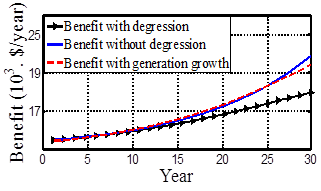
Figure 10. Generation growth(about 9.5% peryear) can nuetralizedegression effect and increase the gross benefit.
3.4. Risk Assessment Analysis
Another fact associated with the financial decisions in FIT policies is the probability of insufficient income for RE developer. Insufficient income can be seen from different points of view, one of them is being potential failure to pay the monthly payment of the loan which is received for starting up the renewable project.
Since the capital cost of renewable technologies is very high, it is common practice for the governments to lend a loan to RE developers for purchasing the technologies. This policy not only encourages people to use renewable, but also compel them to expand their technology in an effective way to reduce the risk of failure to pay the monthly payment of the loan. This risk is defined asthe RE developer risk or RER index.The RER index is dependent on the amount of FIT payment, market price, and generation conditions. Raising the FIT payment or the electricity price as well as improving the generation will result in decreasing the risk of failure to pay back the loan. Thus, it is imperative to decide on a proper amount of FIT payment, parameter![]() , to have an acceptable payback period and small enough RER index.
, to have an acceptable payback period and small enough RER index.
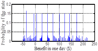
Figure 11. Probability density function of daily benefit.
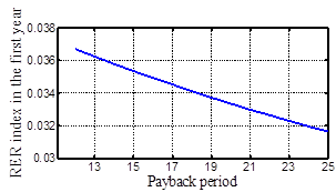
Figure 12. RER index in the first year of the project in terms of payback period.
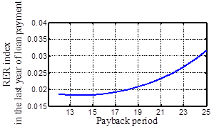
Figure 13. RER index in the last year of the loan payment in terms of payback period.
In the following analysis, the duration of the loan is assumed to be equal (or proportional) to the payback period of the project. It means that if the government chooses an incentive FIT policy to lower the payback period, then the duration of paying the loan alsogets lower.Assume that the amount of loan for the yearly interest rate of 2% equals to the renewable technology capital cost of 233600$, the monthly interest rate is aprroxiamtly
![]() (7)
(7)
Thus, the monthly payment,![]() of the loan can be written in terms of the loan duration as shown below.
of the loan can be written in terms of the loan duration as shown below.
![]() (8)
(8)
Accordingly, different values of payback periods result in various range of loan duration, ![]() and consequently different amount of monthly payments.The daily Markov model for the project gives us the probability of a valid amount of benefit or cost of RE developer in each day. These states and their respective probabilities can be seen as the daily probability distribution function (PDF) of the benefit and cost of the developer, which is shown in Fig. 11. By considering the fact that monthly cost and benefit of the RE developer is sum of the 30 daily costs and benefits, and the obtained daily PDF function for all days are the same, thenthe monthly PDF function in terms of the daily PDFsfunctions is [13]:
and consequently different amount of monthly payments.The daily Markov model for the project gives us the probability of a valid amount of benefit or cost of RE developer in each day. These states and their respective probabilities can be seen as the daily probability distribution function (PDF) of the benefit and cost of the developer, which is shown in Fig. 11. By considering the fact that monthly cost and benefit of the RE developer is sum of the 30 daily costs and benefits, and the obtained daily PDF function for all days are the same, thenthe monthly PDF function in terms of the daily PDFsfunctions is [13]:
![]() (9)
(9)
where "*" denotes the convolution integral of the two functions. After obtaining the probability distribution function of monthly cost and benefit of the RE developer, the RER index is determined as follows:
![]() (10)
(10)
The parameter ![]() in (8) is equal to monthly payment of the loan defined in (8).Fig. 12 andFig. 13 illustrate the RER index for the first and last years of the loan period in terms of the payback period. According to these figures, in the first year RER decreases when the payback period increases; however, in the last year of loan payment (which is equal to the payback period in this study) the RER is a convex function ofthe payback period. Consequently, it is necessary to decide on a policy with appropriate enumeration payment that results in proper payback period and RER index for the total loan payment period. In this case, as Fig.11 and Fig. 12 represent, a suitable value for the parameter
in (8) is equal to monthly payment of the loan defined in (8).Fig. 12 andFig. 13 illustrate the RER index for the first and last years of the loan period in terms of the payback period. According to these figures, in the first year RER decreases when the payback period increases; however, in the last year of loan payment (which is equal to the payback period in this study) the RER is a convex function ofthe payback period. Consequently, it is necessary to decide on a policy with appropriate enumeration payment that results in proper payback period and RER index for the total loan payment period. In this case, as Fig.11 and Fig. 12 represent, a suitable value for the parameter ![]() can be chosen within 50% to 60% which yields payback period from 17 to 21 years, and the RER index within 3.3% to 3.43%in the first year and 1.8% to 2.3% in the last year of the loan payment, respectively. This analysis can help the policy makers to evaluate various premiums and select the best one according to both the government and the RE developer's viewpoints. By choosing this value as the FIT payment, the payback period becomessufficiently small, while the RER index will be small in the first and last years of the loan.
can be chosen within 50% to 60% which yields payback period from 17 to 21 years, and the RER index within 3.3% to 3.43%in the first year and 1.8% to 2.3% in the last year of the loan payment, respectively. This analysis can help the policy makers to evaluate various premiums and select the best one according to both the government and the RE developer's viewpoints. By choosing this value as the FIT payment, the payback period becomessufficiently small, while the RER index will be small in the first and last years of the loan.
4. Conclusion
FIT policies promise great encouragement for REdevelopers in order to increase their generation as well as to make renewable sources a major supply of energy.This paper introduces a noble technique based on Markov state theory to predict load, generation and electricity price behavior. Simulation results approve high potential of the technique in order to design and analyze different types of FIT policies.In summary, the proposed method can be used todesign a model for electricity price and prediction of future behavior of the market. This model can be in terms of hour, day, week, month and year depending on the goals and required accuracy of the analysis. It can be used to design a model of cost and benefit of RE plants inboth net and gross FIT policies, and to examine the RE developer risk in various circumstances for example in project loan payments. This method can also be utilized to compare various FIT policies in order to determine the best choice for a certain country. Furthermore, the influence of unexpected variations in market price, inflation rate, etc. can be added in the models. The method can be applied for the scenarios with more than one RE developers with different types of RE technologies.
References
- T. J. Hammons, J. C. Boyer, S. R. Conners, M. Davies, M. Ellis, and M .Fraser, "Renewable energy alternatives for developed countries,"IEEE Transactions onEnergy Conversion, Vol. 15, pp.481-493, Dec. 2000.
- A. Ameli, S. Bahrami, F. Khazaeli, M.R. Haghifam, "A Multiobjective Particle Swarm Optimization for Sizing and Placement of DGs from DG Owner's and Distribution Company's Viewpoints," Power Delivery, IEEE Transactions on , vol.29, no.4, pp.1831-1840, Aug. 2014
- S. Bahrami, M. Parniani, "Game Theoretic Based Charging Strategy for Plug-in Hybrid Electric Vehicles," Smart Grid, IEEE Transactions on , vol.5, no.5, pp. 2368-2375, Sept. 2014
- R. Haas, C. Panzer, G. Resch, M. Ragwitz, G. Reece, and A. Held, "A historical review of promotion strategies for electricity from renewable energy sources in EU countries,"Renewable and Sustainable Energy Reviews Journal, Vol. 15, pp. 1003–1034, Feb. 2011.
- J. Lipp," Lessons for effective renewable electricity policy from Denmark, Germany and the United Kingdom," Energy Policy Journal, Vol.35 (11), pp. 5481–5495, Nov. 2007.
- C. Mitchell, "The renewable NFFO, A review," Energy Policy Journal, Vol. 23(12), pp. 1077-1091, 1995.
- E. Holt, "The role of renewable energy certificates in developing new renewable projects," National Renewable Energy Laboratory, Colorado, Tech. Rep. NREL/TP-6A20-51904, June 2011.
- M. Ringel, "Fostering the use of renewable energies in the European Union: the race between feed-in tariffs and green certificates,"Renewable Energy Journal, Vol. 31 (1), pp. 1–17.Jan. 2006.
- S. Wong, K. Bhattacharya, and J. D. Fuller, "Long-term effects of Feed-In Tariffs and carbon taxes on distribution systems,"IEEE Transaction on Power Systems, Vol. 25, Aug. 2010.
- A. Pollock and E. McNamara, "What Is an Effective Feed-In Tariff for Your State? A Design Guide," National Regulatory Research Institute,Vol. 10, pp.1-10, Apr. 2010.
- P. D. Rio and M. A. Gual, "An Integrated Assessment of Feed In Tariff System in Spain," Energy Policy Journal, Vol. 35, pp. 994-1012, Feb. 2007.
- A. Zahedi, "A review on feed-in tariff in Australia, what it is now and what it should be," Renewable and Sustainable Energy Reviews, Vol. 14, pp. 3252-3255, Jan. 2010.
- T. Couturen and Y. Gagnon, "An analysis of feed-in tariff remuneration models: Implications for renewable energy investment," Energy Policy Journal, Vol.38, pp. 955-965, Feb 2010.
- F. Muhammad-Sukki, R. Ramirez-Iniguez, S. H. Abu-Bakar, S. G. McMeekin, and B. G. Stewart, "Feed-In Tariff for solar PV in Malaysia: Financial analysis and public perspective,"International Power Engineering and Optimization Conference (PEOCO), pp. 221-226, 2011
- L. Dusonchet and E. Telaretti, "Economic analysis of different supporting policies for the production of electrical energy by solar photovoltaic's in eastern European Union countries," Energy Policy Journal, Vol. 38, pp. 4011-4020, Jan. 2010.
- J. A. Lesser and X. Su, "Design of an economically efficient feed-in tariff structure for renewable energy development," Energy Policy Journal, Vol.36, pp. 981-990, Mar. 2008.
- G. Shrimali and E. Baker, "Optimal Feed-in Tariff schedules," IEEE Transaction on Engineering Management, Vol.59, pp. 310-322, May. 2012.
- I. Ritzenhofen and S. Spinler, "Optimal design of feed-in-tariffs to stimulate renewable energy investments under regulatory uncertainty — A real options analysis," Energy Economics, Dec. 2014.
- N. Martin and J. Rice, "The solar photovoltaic feed-intariff scheme in New South Wales, Australia," Energy Policy, Vol.61, pp.697-706. Oct. 2013.
- R. Billinton and R. N. Allan, "Reliability evaluation of engineering system," Plenum press, New York, 1996.
- R. BillintonandR.N.Allan, "Reliability evaluation of power system," Plenum press, New York, 1996.
- J.D. Hall, R. J. Ringlee, and, and A. J. Wood, "Frequency and duration methods for power system reliability calculations,Part I, Generation system model,"IEEE Transaction on Power Apparatus and System,Vol. 87,pp. 1787-1779, Sept.1968.
- J.D. Hall, R. J. Ringlee, and A. J. Wood, "Frequency and duration methods for power system reliability calculations, Part II, Demand model and capacity reserve model', IEEE Transaction on Power Apparatus and System, Vol. 88, pp. 375-388, Apr. 1969.
- R. Billinton and C. Singh, "System load representation in generating capacity reliability studies," IEEE Transaction on Power Apparatus and Systems, Vol. 91, pp. 2125 – 2132, Sept. 1972.
- Australian Energy Market Operator (AEMO), 2014, Online: Available: http://energy.anero.id.au/wind-energy
- http://windfarmperformance.info/


