Numerical Modeling of the Breakup Mechanism of Liquid Ligaments in Two-Phase Flow Application Using Level Set Method

Ashraf Balabel^*

Mechanical Engineering Dept., Faculty of Engineering, Taif University, Al-Haweiah, Taif, Saudi Arabia

Abstract

The present paper introduces a numerical modeling for one of the most important problems of two-phase flows; namely the breakup mechanism of stretched liquid ligaments. The challenge problem of such complex flow is how to deal with the breakup of liquid ligaments in natural way without any constraints or numerical instability. The present modeling is based on solving the governing equations of motion in the liquid phase by the aid of the control volume strategy on a non-sta-ggered grid system. The level set function is further applied to track and capture the moving interface by using the normal velocity components located directly at the liquid interface. Some numerical test cases are performed to indicate the ability of the proposed numerical method in predicting the breakup mechanism of liquid ligaments. The obtained results showed that the developed numerical method is capable of simulating the formation and the breakup mechanism of the ligaments formed in two-phase flows without any numerical constraints.

Keywords

Breakup Mechanism, Liquid Ligaments, Level Set Method, Numerical Modeling, Two-Phase Flow Dynamics

Received: May 20, 2015
Accepted: June 6, 2015
Published online: July 15, 2015

@ 2015 The Authors. Published by American Institute of Science. This Open Access article is under the CC BY-NC license. http://creativecommons.org/licenses/by-nc/4.0/

1. Introduction

The separation and breakup of liquid ligaments are considered as the most challenging topic of the numerical simulation of two-phase flows [1]. That can be seen in numerous industrial and engineering applications, e.g., atomization and spray of liquid jet [2], bubble and droplet dynamics [3], and other multiphase flow systems [4].

Numerical simulations have recently become an important tool for predicting and understanding many engineering processes. The mean feature of such engineering processes is the moving interface between the two phases. This moving interface can be advected by the normal velocity components on the separating surface according to the existed interfacial boundary conditions. The advection process may be a linear or a nonlinear regime according to the included terms in the governing equations. In the nonlinear regimes, there is a few numbers of developed methods for solving the governing equations [5,6]

The most general methods for treating two-phase flows with moving interfaces are boundary integral formulations [7] and further applications in [8]. Many incompressible flow algorithms have been used to solve the two-phase flow problems accompanied by a suitable surface tracking method. As mentioned in [9], both of conventional conservative and high order conservative schemes can produce excessive numerical diffusion and oscillations which destroy the smoothness of the front. That can be seen in [10]. Another scheme is based on the projection method developed in [11], and it has been combined along with the level set to simulate two-phase flows, e.g. [12]. In conclusion, a truly general method is not yet available [13].

A great challenge in the numerical simulations of unsteady motion of two-phase flows is how to predict the topological change of the interface because the motion is very sensitive to small numerical perturbations, such as merging and breaking of the interface. Many techniques have been used to deal with the propagation of the interface in two-phase flows. These techniques are based basically on two different approaches: the Lagrangian approach and the Eulerian approach see for more details [14-17].

Based on the Eulerian approach, another technique has been used in [9]. This technique is based on tracking the interface using a grid that moves through a stationary Eulerian grid. Here complication occurs when one needs to add or subtract points to the moving grid. The major limitation of this method is the treatment of interfaces that interact. Moreover, these problems are become important when solving a three dimensional problem. Another example for moving grid technique is used in [18]. In this technique the fluid is bounded by a height function varying with time along the fluid interface. This function determines the radial distance through evolution. This algorithm is limited to a case in which the interface does not overturn, see for more details [19].

Two types of methods are available and widely used; the Volume-Of-Fluid (VOF) methods [20,21] and the Level Set methods [22]. These methods avoid explicitly tracking the interface, and consequently, avoiding many of the topological limitations.

The level set method, unlike the VOF method, divides the solution domain containing the two phases into a region where a scalar quantity, say, is smaller or larger than a fixed value f₀. The value of the level set function f is assigned to each grid point in the calculation domain, thereby determining whether it belongs to the liquid or the gas phase. The level set method is widely applied in two-phase flows applications, e.g. [25,12] and more recently in [26-33].

2. Mathematical Formulations

The governing equations for incompressible two-phase flow are mathematically expressed by the conservation equations of the mass and momentum at each point of the flow field. These equations can be written in the primitive variables formulation in form of continuity equation and Navier-Stokes equations, respectively, as follows:

                                          (1)

              (2)

Where r, u, p, m are the density, velocity vector, pressure and viscosity of the fluid. The subscript i denotes the liquid phase (i=1) and the gas phase (i=2), respectively

The coupling between the pressure and velocity field is made through the Poisson equation for pressure:

                  (3)

The Poisson equation is solved by the Successive Over-Relaxation method in each phase to obtain the pressure in the considered phase.

2.1. Computational Methodology

The so-called implicit fractional step-non iterative method is applied in our present work by presuming that the velocity field reaches its final value in two stages;

                                   (4)

Whereby,  is an imperfect velocity field based on a guessed pressure field, and  is the correction velocity. The 'starred' velocity will be obtained from solving of the momentum equations. After that, the solution of Poisson equation for the pressure:

                             (5)

where  will be called the pressure correction.

The velocity correction is obtained according to:

                                (6)

This fractional step method described above ensures the proper velocity-pressure coupling for incompressible flow fields [32].

2.2. Level Set Method

In absence of the interfacial mass transfer such as evaporation or condensation, the equation of the level set method can be written as:

                             (7)

And from the level set function, the normal vector and the interface curvature can be calculated as:

                         (8)

It should be pointed out that, the curvature of the interface is calculated only on the main grid points. However, the exact curvature should be calculated at the interfacial markers located on the intersection points of the computational grid with the interface. Consequently, the interpolation scheme applied for obtaining the fluid variables at the interface is also applied for calculating the interfacial curvature, for more details one can see [27]

In another form of the level set method, where the normal velocity component is included, the level set equation becomes

                               (9)

By further manipulation, the normal velocity is replaced by the velocity field F_ext known as the extension velocity, which at the zero level set, equals the given speed V_n. In other words, the level set equation can be written as:

                            (10)

Where,

                               (11)

The above equation is solved by using the second-order Runge-Kutta method and the overall domain is re-initialized each time step [27].

2.3. Interfacial Boundary Conditions

The boundary conditions at the interface, or jump conditions, may be written in the following general form:

                (12)

Where I is the identity matrix, p is the pressure, m is the dynamic viscosity, s is the surface tension coefficient, and D is the rate of deformation tensor. The bracket means the jump of the stresses along the fluid interface G, the unit normal vector n is taken from fluid 2 to fluid 1,denotes the gradient in the local free surface coordinates, and t is an arbitrary vector perpendicular to the normal of the interface. The curvature of the interface k is computed from the following equation:

                                     (13)

In contrast to the previous two-phase numerical methods, in which the interfacial jump conditions are embedded naturally on the momentum equations by applying CSF model [35], the jump conditions between the two fluids are treated here as a boundary conditions enforced explicitly at the interface G.

The above interfacial boundary equation, Eq. (12) can be written in the normal and tangential directions, respectively:

                        (14)

                      (15)

The kinematic conditions are satisfied by assuming the continuity of the normal velocity components, i.e.

                                   (16)

In addition to that, the liquid gas interface requires equality of dynamic stresses, especially shear stresses, on both sides of the interface, i.e.

                                        (17)

The system of the above equations and the prescribed boundary conditions should be solved simultaneously to determine the flow field in the two fluids. The normal velocity components are then used for the advection of the interface by solving the appropriate equation of the level set function.

3. Results and Discussions

The first test case performed using the above developed numerical method is the falling of a water droplet from a pipette with specified dimensions and with a constant initial velocity. The sequence of the pictures presented shows that the droplet is firstly formed from a nearly sinusoidal wave form initiated at the open side of the pipette. Under the effect of the initial velocity, the droplet is formed and a thin ligament is shown to connect the droplet with the liquid inside the pipette. At the last stages of the simulation the droplet detaches from the liquid surface and a single droplet moves under the gravity downward.

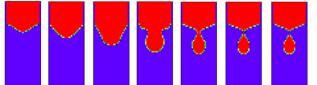
Figure 1.A sequence of pictures of a drop of water falling from a pipette.

From the above results, it can be shown that the formation of the ligament and the breakup of the single droplet are carried out in natural way without any numerical instabilities or constraints.

The second performed test case shows the breakup mechanism of an elongated droplet with initial ellipsoid shape under the surface tension effects only. The deformation of the droplet is started according to the nonlinear theory of droplet deformation. At later steps of the simulation, two satellite droplets and a mother droplet can be observed. As in the previous example, the breakup mechanism is carried out without any numerical problems.

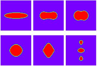
Figure 2.A sequence of breakup mechanism of an elongated drop under surface tension effects.

4. Conclusions

In the present paper, the numerical modeling of the formation of liquid ligament and the further breakup of the liquid droplet is carried out. The numerical method developed is based on solving the momentum equations coupled with the level set method. The obtained results showed a remarkable capability of the developed numerical method in predicting the formation and the further breakup of the ligaments and satellite droplets without any numerical constraints. This encourages us to further include a wide range of two-phase flow industrial and engineering applications.1

References

1. Linne M., Paciaroni M., Hall T., and Parker T., Ballistic imaging of the near field in a dense spray", Exp. Fluids., 49(4): 911-923, 2006.
2. Lefebvre, A. H., Atomization and sprays, Hemisphere Publishing Corporation, 1989.
3. Fuster, D., Agbaglah, G., Josserand, C., Popinet, S. and Zaleski, S., Numerical simulation of droplets, bubbles and waves: state of the art, Fluid Dyn. Res. 41: 1-24, 2009.
4. Kolev N.I., Multiphase flow dynamics: Thermal and Mechanical Interaction", Springer, 2007.
5. Eggers, J. Nonlinear Dynamics and Breakup of Free-Surface Flows. Reviews  Modern Physics., 69, No.3, 1997.
6. Eggersand, J., Dupont, T., Drop Formation in a one-dimensional Approximation of the Navier-Stokes equation, J. Of Fluid Mech., vol.262, pp. 205-221, 1994.
7. G.K. Youngern and A. Acrivos. On the Shape of the Gas Bubble in a viscous Extensional Flow. J. of Fluid Mech., vol. 76, pp. 433-442, 1976.
8. J. M. Rallison and A. Acrivos. A Numerical Study of the Deformation and Burst of a Viscous Drop in an Extensional Flow. J. of Fluid Mech., vol. 89, pp. 191-200, 1978.
9. S. O. Unverdi and G. Traggvason. A Front-Tracking Method for Viscous, Incomprissible Multi-Fluid Flows. J. Comp. Phys., 100, 25-37, 1992.
10. R. Sandra and H. Philippe. Mathematical and Numerical Modeling of a Two- Phase Flow by a Level Set Method. Proc. Finite Volumes for Complex applications II, 1999.
11. J. Bell and D. Marcus. A Second-Order Projection Method for Variable-Density Flows. J. Comp. Phys., 101, 334-348, 1992.
12. M. Sussman, P. Smereka, and S. Osher. A Level Set Approach for Computing Solutions to Incompressible Two-Phase Flow. J. Comp. Phys., 114, 146-159, 1994.
13. W.-T. Tsai and D. K. P. Yue. Computation of Nonlinear Free-Surface Flows. Annu. Rev. Fluid Mech., 28, 249, 1996.
14. B.J. Daly. A Technique for Including Surface Tension E_ects in Hydrodynamic Calculation. J. Comp. Phys., vol. 4, pp. 97-117, 1969.
15. J.E. Welch, F.H. Hrlow, J.P. Shannon, and B.J. Daly. The MAC-Method: A Computing Technique for Solving Viscous, Incompressible, Transient Fluid Flow Problems Involving Free Surfaces. Los Alamos Sci. Lab. Rep. LA-3425, 1966.
16. R. Cortez. An Impulse-Based Approximation of Fluid Motion due to Boundary Forces. J. Comp. Phys., 123, 341-353, 1995.
17. H. A. Stone and L. G. Leal. Relaxation and Breakup of an Initially Extended Drop in an Otherwise quiescent Fluid . J. Fluid Mech., vol. 198, 399-427, 1989.
18. F. Mashayek and N. Ashgriz. A Height-Flux Method for Simulating Free Surface Flows and Interfaces. Int. Num. Meth. in Fluids, vol. 17, pp. 1035-1054, 1993.
19. R. M. Schulkes. The Evolution and Bifurcation of a Pendant Drop. J. of Fluid  Mech., vol. 278, pp. 83-100, 1994.
20. C.W. Hirt and B.D. Nichols. Volume of Fluid method (VOF) for the Dynamics of Free Boundaries. J. Comp. Phys. vol. 39, pp. 201-225, 1981.
21. S. Zaleski, J. Li, and S. Succi. Two-dimensional Navier-Stokes Simulation of Deformation and Break-up of Liquid Patches. Phys. Rev. Lett., vol.75, pp.244-247, 1995.
22. J.A. Sethian. An Analysis of Flame Propagation. Ph.D. Dissertation, Mathematics, Uni. of California, Brekeley, 1982.
23. B. Lafaurie and et al. Modelling Merging and Fragmentation in Multiphase Flows with SURFER. J. Comp. Phys., 113, 134-147, 1994.
24. Th. Schneider and R. Klein. Overcoming mass losses in Level Set-based interface tracking schemes. Proc. Finite Volumes for Complex applications II, 1999.
25. K. Naitoh and Y. Takagi. OPT Model for Fuel Atomization behavior. Proc. Of Commodia 94, 1994.
26. Balabel A. (2013): Numerical Modelling of Liquid Jet Breakup by Different Liquid Jet/Air Flow Orientations Using the Level Set Method, Computer modeling in engineering & sciences, vol. 95 (4), pp. 283-302.
27. Balabel, A.; El-Askary, W. (2011): On the performance of linear and nonlinear k–e turbulence models in various jet flow applications. European Journal of Mechanics B/Fluids, vol. 30, pp. 325–340.
28. Balabel, A. (2011): Numerical prediction of droplet dynamics in turbulent flow, using the level set method. International Journal of Computational Fluid Dynamics, vol. 25, no. 5, pp. 239-253.
29. Balabel, A. (2012): Numerical simulation of two-dimensional binary droplets collision outcomes using the level set method. International Journal of Computational Fluid Dynamics, vol. 26, no. 1, pp. 1-21.
30. Balabel, A. (2012): Numerical modeling of turbulence-induced interfacial instability in two-phase flow with moving interface. Applied Mathematical Modelling, vol. 36, pp. 3593–3611.
31. Balabel, A. (2012): A Generalized Level Set-Navier Stokes Numerical Method for Predicting Thermo-Fluid Dynamics of Turbulent Free Surface. Computer Modeling in Engineering and Sciences (CMES), vol. 83, no.6, pp. 599-638.
32. Balabel, A. (2012): Numerical Modelling of Turbulence Effects on Droplet Collision Dynamics using the Level Set Method. Computer Modeling in Engineering and Sciences (CMES), vol. 89, no.4, pp. 283-301.
33. Balabel, A. (2013): Numerical Modelling of Liquid Jet Breakup by Different Liquid Jet/Air Flow Orientations Using the Level Set Method. Computer Modeling in Engineering and Sciences. (CMES), Vol. 95, No. (4), pp. 283-302.
34. Sethian, J. A. and Smereka, P., Level set methods for fluid interfaces, Annu. Rev. Fluid, Mech., 35, 341-372, 2003.
35. Brackbill, J. U., Kothe, D. B. and Zemach. A,, A Continuum Method for Modeling Surface Tension, J. Comp. Phys., 100 (1992) 335-354.