
American Journal of Geophysics, Geochemistry and Geosystems, Vol. 1, No. 2, June 2015 Publish Date: Apr. 22, 2015 Pages: 19-36
Geomorphological Interpretation Through Satellite Imagery & DEM Data
Kuldeep Pareta1, *, Upasana Pareta2
1RS/GIS & NRM, Spatial Decisions, New Delhi, India
2Mathematics, P.G. College, District - Sagar, Madhya Pradesh, India
Abstract
In this paper, the geological aspect, topographic characteristics, hypsometric analysis and geomorphological characteristic of the Pench reserve area is analysed and described by DEM data, and multi-temporal, multi-sensors, multi-spectral, & multi-resolution satellite remote sensing imageries. Based on the digital elevation model (SRTM-DEM, ASTER-DEM, CartoSAT-DEM) data, LandSAT imageries i.e. LandSAT-7 ETM+ data & LandSAT-8 OLI data, IRS imagery i.e. ResourceSAT-2 LISS-III data and 1:50,000 topographic map data, a comprehensive analysis and study on the geomorphology and topography of the Pench reserve area was conducted using such means as data pre-processing, interpretation and mapping, on the software platforms including ESRI ArcGIS-10.3, and ERDAS Imagine-2013, which aided a better option for visualizing the terrain and mapping. This observations and analysis are able to improve by measure, monitor and analysis forms of terrain using by satellite imagery and DEM data. Using both DEM and remote sensing together open new dimension on earth sciences and investigation topographic and geomorphological characteristics of the landforms.
Keywords
Geomorphology, Topography, Hypsometric Analysis, Remote Sensing, GIS, and Pench Area
Received: April 9, 2015
Accepted: April 12, 2015
Published online: April 20, 2015
@ 2015 The Authors. Published by American Institute of Science. This Open Access article is under the CC BY-NC license. http://creativecommons.org/licenses/by-nc/4.0/
Contents
1. Introduction 2. Study Area 3. Data Selection and Processing 3.1. Data Sources 3.2. Data Selection 3.3. Elevation Data 3.4. Remote Sensing Image Data 3.5. Data Processing 4. Geology 4.1. Tirodi Biotite-Gneiss Formation 4.2. Sausar Group 4.3. Lohangi Formation 4.4. Chorbaoli Formation 4.5. Lametas / Infra-Trappean Series 4.6. Deccan Traps 4.7. Inter-Trappean Beds 4.8. Alluvium and Laterite 5. Geomorphology 6. Topographic Characteristics 7. Hypsometric Analysis 7.1. Hypsometric Integrals 7.2. Practical Applications of Hypsometric Analysis 8. Conclusion Acknowledgment
1. Introduction
Geomorphology is the study of landforms and landscapes, including the description, classification, origin, development, and history of planetary surfaces (Salisbury, 1907).Quantitative geomorphological analysis can provide the information about landscapes evolution & development, shape and dimension, surface processes and the behavior of surface drainage networks. Rai (1969), Pal (1973), Singh (1991), Fuli (1993), Mohanty (1993), Khan et al, (1999), Tiwari (2001), Rao (2002), Ray & Chakraborty (2002), Jain et al, (2008), Ramteke et al, (2012), and Naithani et al, (2014) had made some relevant research efforts on the geochronology and geology in this area, but the research data are still short as a whole.In recent years, with the quick development of remote sensing technology, geographic information system and global positioning system, many researchers have started to extract and interpret the geomorphological features with DEM data, remote sensing images and other image information. A number of inventors have contributed to explore the geomorphological aspects through the GIS and satellite remote sensing techniques. Notable these are Fairbridge (1968), Rao (1975), Verstappen (1977), Curran et al, (1984), Baker (1986), Hayden et al, (1986), Short et al, (1986), Jenson et al, (1988), Krishnamurthy et al, (1995), Way et al, (1997), Sabins (1997), Colwell (1997), Rao (2002), Yokoyama et al, (2002), Reddy et al, (2003), Mith et al, (2005), Drăguţ et al, (2006), Blaschke (2010), Pareta et al, (2011), etc.
In this paper, the geological aspect, topographic characteristics, hypsometric analysis and geomorphological characteristic of the Pench reserve area were extracted and interpreted through processing of the SRTM-DEM data, ASTER-DEM data, CartoSAT-DEM data, LandSAT’s and ResourceSAT satellite image data, and 1:50,000 topographic map using such applications as ESRI ArcGIS-10.3 &ERDAS Imagine 2013, and with previous literature review, and published geological map. Furthermore, in the study area so far not any systematic and scientific work on the geomorphology has been carried out making the present study a necessary aim.
2. Study Area
The study area situated in reserve and protected forests of south Seoni division in Seoni district and south-east Chhindwara divisions of Chhindwara district, between 21.62 to 21.95 N latitudes and 78.95 to 79.53 E longitudes covering an area of 1024.59 Kms2. The study area falls under the Survey of India Topo Sheet (1:50,000 Scale) No. No.: 55K/13, 55K/14, 55O/01, 55O/02, 55O/05, 55O/06, and 55O/09. According to Govt. of M.P. Forest Department's Notification No. F.15-31-2007-X-2, dated: 24th December 2007, an area of 411.33 Kms2 of Indira Priyadarshini Pench National Park and Pench Mowgli Sanctuary was declared as core area of Pench tiger reserve. Out of that 292.85 Kms2area fall under the Indira Priyadarshini Pench National Park, and 118.47 Kms2areas fall under the Pench Mowgli Sanctuary (Fig. 1).

Figure 1. Location map of the study area
Physiographically, the area is undulating; it can divide in four region i.e. north & north-eastern hilly region, central high plateau region, south & south-eastern low grounds, and upland trough of Pench river. Pench River and its tributaries are flowing in this area. Pench reservoir is also situated in the area. Primarily the underlying rocks govern the drainage system in the area. The drainage pattern is generally dendritic type. The study experiences a hot summer and general dryness characterize the climate, except during the south-west monsoon season. Rain occurs due to the south-west monsoon winds from June to September. The average annual rainfall is about 1317 mm, bulk of which is received during monsoon months of June to September, about 85% of the annual rainfall falls. The normal maximum temperature noticed during the month of May is 39.4oC and minimum during the month of December 9.8oC. The normal annual mean minimum and maximum temperatures has been worked out as 18.2oC and 30.6oC respectively.
3. Data Selection and Processing
3.1. Data Sources
Table 1. Data used and sources
| S.No. | Data Used | Sources |
| 1. | SoI Toposheets @ 1:50,000 Scale | Survey of India, Dehradun No.: 55K/13, 55K/14, 55O/01, 55O/02, 55O/05, 55O/06, and 55O/09 |
| 2. | Indian Topographic Map @ 1:250,000 | Series U502, U.S. Army Map Service, 1955 http://www.lib.utexas.edu/maps/ams/india No.: NF 44-09 and NF 44-10 |
| 3. | Shuttle Radar Topography Mission (SRTM), DEM Data @ 90m Spatial Resolution | NASA, & USGS EROS Data Center, 2006 http://glcfapp.glcf.umd.edu:8080/esdi |
| 4. | ASTER Global Digital Elevation Model (GDEM), DEM Data @ 30m Spatial Resolution | Japan Space Systems (J-space systems) Japan, cooperation with US, 2009 http://gdem.ersdac.jspacesystems.or.jp/search.jsp |
| 5. | CartoSAT-1 Digital Elevation Model (CartoDEM), DEM Data @ 30m Spatial Resolution | Indian Earth Observation, National Remote Sensing Centre (ISRO), India http://bhuvan.nrsc.gov.in/data/download/index.php Date: 02nd December, 2007(Grid: F44N & F44M) |
| 6. | LansSAT-7 ETM+ (Enhance Thematic Mapper ) Data @ 30m Spatial Resolution | Global Land Cover Facility (GLCF) http://glcfapp.glcf.umd.edu:8080/esdi/ Date: 11th November, 2000 (Path: 144, Row: 45) |
| 7. | IRS ResourceSAT-2 LISS-III Data @ 23.5m Spatial Resolution | Indian Earth Observation, National Remote Sensing Centre (ISRO), India http://bhuvan.nrsc.gov.in Date: 04th November, 2011 (Grid: F44N & F44M) |
| 8. | LandSAT-8 OLI (Operational Land Imager) Data @ 30m Spatial Resolution | U.S. Geological Survey, Earth Resources Observation & Science Center (EROS) http://earthexplorer.usgs.gov Date: 14th February, 2015 (Path: 144, Row: 45) |

Figure 2. ASTER (DEM) data
3.2. Data Selection
Since the purpose of this paper was to interpret the geomorphological analysis, which had a large area and contained abundant information, the data employed in this paper were dominated by the freely downloaded elevation data and remote sensing image data, whose accuracy achieved the interpretation requirements and whose amount was relatively small to facilitate processing. The study area has a large distribution area, and it is located in reserve and protected forests, with undulating surface including valley, bed land, denudational / residual / structural hill, plateau, dissected valley slope, pediment and plain that are evenly distributed and less interfered with by other geologic bodies, so both the elevation data and remote sensing image data were combined to extract the spatial information and spectral information of the study area in this paper.
3.3. Elevation Data
3.3.1. Digital Elevation Model (DEM) Data
The data were from Shuttle Radar Topography Mission (SRTM), NASA, & USGS EROS Data Center (spatial resolution 90m), ASTER Global Digital Elevation Model (GDEM) (Fig.2), Japan Space Systems (J-space systems) Japan, cooperation with US, and Cartosat-1 Digital Elevation Model (CartoDEM) (Fig. 3), Indian Earth Observation, National Remote Sensing Centre (ISRO), India - geospatial data cloud, with projection coordinates of UTM/WGS-84 and spatial resolution of 30 m, and were used to display the elevation undulation.

Figure 3. CartoSAT-1 (DEM) data

Figure 4. Topographic data

Figure 5. LandSAT-8 OLI satellite imagery, 2015

Figure 6. IRS ResourceSAT-2 LISS-III satellite data, 2011
3.3.2. 1:50,000 Topographic Data
The data were from Survey of India topographical maps No. 55K/13, 55K/14, 55O/01, 55O/02, 55O/05, 55O/06, and 55O/09, with a contour interval of 20 meters, and freely available topographic map at 1:250,000 (NF 44-9 and 10) (Fig. 4) from Series U502, U.S. Army Map Service, 1954 with a contour interval of 30 meters. The data were mainly used for extraction of the hypsometric parameters and analysis of the morphological characteristics of the study area.
3.4. Remote Sensing Image Data
3.4.1. LandSAT Remote Sensing Data
The data were from the LandSAT-8 OLI (Operational Land Imager) satellite launched by National Aeronautics and Space Administration (NASA) of USA has been downloaded from U.S. Geological Survey, Earth Resources Observation & Science Center (EROS). In order to enhance the display of the study area, the images with low cloud content acquired in 14th February, 2015 were used in this paper (Fig. 5). The data covered 11 bands in total, with spatial resolutions as follows: OLI multispectral band (30 meters); OLI panchromatic band (15 meters); and TIRS band (30 meters); UTM WGS-84 projection coordinate system. The data were used to extract the geology, geomorphic unit and analyse the spectral characteristics of the area.
3.4.2. IRS ResourceSAT-2 LISS-III Data
The data were from the IRS ResourceSAT-2 LISS-III by Indian Earth Observation, National Remote Sensing Centre (ISRO), India was captured on 04th November 2011 was also used. The data covered 4 bands in total with spatial resolutions of 23.5 meters. The data (Fig. 6) were used as the same purposed as described above.
3.5. Data Processing
The original image data were combination of all kinds of information, and contained much information. Due to the different coordinate projection systems, the image data should be pre-processed and enhanced to extract some geographic elements. The contrast between the study area and the background was enhanced through the computation of image data, thus to extract special geomorphologic parameters.
3.5.1. Elevation Data Processing
The elevation data mainly included the DEM data and the topographic map data. The elevation data processing steps were as follows: (i) conduct pre-processing such as defining coordinate system, image registration, image correction and cropping for the selected area; (ii) generate corresponding slope map, aspect, hillshade, and viewshed map with the pre-processed data, and extract contour lines; (iii) carry out layer operation, reclassification and weighted overlaying processing of the generated slope map, and elevation / physiography map; (iv) prepared three-dimensional map (Fig. 7).

Figure 7. Three-dimensional view of the study area
3.5.2. Remote Sensing Data Processing
In this paper, the pre-processing operations such as image registration, correction and cropping, of multi-spectral image data were conducted mainly using the ERDAS Imagine-2013, and then the spatial resolution of image was improved through inter-band fusion, and the image was enhanced through false color composite and linear stretching, to highlight relevant thematic information; finally, with the field exploration results being taken into account, visual interpretation was made, to extract relevant thematic information. The specific data processing flow chart is shown in Fig. 8).
4. Geology
Satellite remote sensing imagery based geological map can usually provide the information such as (i) distribution of the rock type and lithological groups in the area. Age cannot be determined from photographs alone, unless prior reference is available about them; (ii) an indication of the dips of the strata, which are classified as gentle, moderate and steep. After some practice a geologist can estimate the actual amount of dip fairly accurately; (iii) faults and unconformities can also be picked up on satellite imagery with fair certainty. In fact, faults are much more easily picked up on satellite imagery than from ground surveys and sometimes, though not always; it is also possible to give their throw and character.
In many countries, geologic maps have been prepared on the basis of few traverses only and, therefore, regional relationships may be wrong. Satellite imagery because of its regional coverage can help to solve this problem by preparing adequate reconnaissance geological maps, for areas where base maps are lacking, which are inaccessible or where ground truth is minimal.
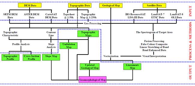
Figure 8. Data processing flow chart
The interpretation of satellite remote sensing data may be best accomplished by visual interpretation techniques with the under-standing of spectral property of earth/ rock materials, and their appearance on the images. Due to climatic impact on weathering, landslide, mass movement, LULC & vegetation cover, image interpretation criteria can be changed from a region to another region.
A general geological map of the area has been prepared by the Geological Survey of India (GSI) through the conventional methods. Several societies have contributed to diverse geological aspects of the region. Remarkable these are Fermor (1909), Bhattacharjee (1922), Buchanan (1923), West (1936), Holmes (1955), Turner and Verhoogen (1960), Straczek et al. (1956), Narayanaswami et al. (1963), Roy and Purkait (1965), Basu and Sarkar (1966), Fyee and Turner (1966), Roy (1966), Agrawal (1968), Subramanyam (1972), Phadke (1990), Mohanty (1993), etc. They have recorded the principal rock formations namely Tirodi Biotite-gneiss formation (biotite gneiss, amphibolite), Lohangi formation (gneisses, marble, and manganese deposits), Chorbaoli formation (quartzite, feldspathic schists, gneisses, and quartz conglomerate), Lametas or infra-trappean series (cherty limestone, shale), Deccan traps (basic dyke basaltic flow with inter trappean beds), and alluvium & laterite (Fig. 9). The general geological succession of the study area is given below:
Table 2. General geological succession of the study area
| Stratigraphic Succession | |||
| Age | Groups & Formations | Lithology / Rock Type | |
| Recent to Cenozoic | Quaternary | Alluvium and Laterite | Silt, Sand, Gravel, Laterite |
| Lower Eocene to Upper cretaceous | Deccan Traps | Basic Dyke Basaltic Flow with Inter Trappean Beds | |
| ~ ~ ~ ~ ~ ~ ~ ~ ~ ~ ~ ~ ~ ~ ~ ~ ~ ~ ~ ~ ~ ~ Slight Unconformity ~ ~ ~ ~ ~ ~ ~ ~ ~ ~ ~ ~ ~ ~ ~ ~ ~ ~ ~ | |||
| Late Cretaceous | Lametas or Infra-Trappean Series | Chert, Cherty Limestone and Shale | |
| Meso-Proterozoic | Sausar Group | Chorbaoli Formation | Quartzite, Feldspathic Schists, Gneisses, Autoclastic Quartz Conglomerate |
| Mansar Formation | Metapelitie (Mica Schist and Gneisses), Graphitic Schist, Phyllite, Quartzite, Major Manganese Deposits and Gondite | ||
| Lohangi Formation | Calc-Silicate Schists and Gneisses, Marble, Manganese Deposits | ||
| ~ ~ ~ ~ ~ ~ ~ ~ ~ ~ ~ ~ ~ ~ ~ ~ ~ ~ ~ ~ ~ ~ Disconformity ~ ~ ~ ~ ~ ~ ~ ~ ~ ~ ~ ~ ~ ~ ~ ~ ~ ~ ~ ~ ~ ~ ~ | |||
| Lower Pre-Cambrian | Tirodi Biotite-Gneiss Formation | Biotite Gneiss, Amphibolite, Calc-Silicate Gneiss, Granulites, Feldspathic, Conglomerate | |
| After Straczek et al. 1956 | |||
4.1. Tirodi Biotite-Gneiss Formation
Tirodi biotite gneiss (TBG) is dominantly a migmatite with components of biotite-muscovite schist, biotite gneiss, hornblende schist and gneiss. Straczek et al. (1956) included this unit within the Sausar Group as the basal member. Narayanaswami et al. (1963) considered the Tirodi gneiss to be the basement of the Sausar Group, with a disconformable relation between the two, on the basis of: (a) gneissic character of the Tirodi biotite gneiss even at the contact of low grade metamorphic rocks of the Sausar Group, (b) presence of more quartz veins and pegmatites in the gneiss than in the Sausar Group, and (c) absence of intense minor cross folds developed in the gneiss inside the Sausar Group (Subramanyam, 1972). However, neither any sedimentological evidence nor any detailed structural analysis to support the idea of the basement-cover relationship has so far been cited. On the other hand, some of the workers in Narayanaswami et al (1963) even considered the possibility of Tirodi gneiss being a product of migmatisation syntectonic with intrusion of granites into the Sausar Group. Phadke (1990) has also expressed a similar view about the relation between the Tirodi gneiss and the Sausar Group. Thus, the question of the relation of the Tirodi gneiss with the Sausar Group has not been solved, but the tacit assumption has been made that the former is the basement of the latter (Mohanty, 1993). Tirodi biotite-gneiss consists of biotite gneiss, amphibolite, calc-silicate gneiss, granulites, feldspathic, conglomerate. These rocks form the basement of all other formation, so they are referred as basement complex or fundamental gneiss. Tirodi biotite-gneiss is found in most parts of the study area, and has covered 60.11% of the area.
4.2. Sausar Group
The Sausar Group (SSG) is also known as the Sausar mobile belt. The work of Bhattacharjee (1922), West (1936), Straczek et al. (1956), Basu and Sarkar (1966) and Agrawal (1968) in different parts of the Sausar belt has established that the rocks of the Sausar group have a polyphase structure history, the successive metamorphic and structure events being assigned to the Satpura orogenic cycle (Holmes 1955). The manganese ore of this area is associated with the rocks of Sausar series. The manganese formation of the Sausar Group were first studied by Fermor (1909), followed by others including Straczek et al. (1956), Narayanaswami et al. (1963) and Roy (1966). The Sausar Group of rocks occur in the area as an arcuate belt, trending NE-SW, E-W and NW-SE from the eastern to the western part. The lithology suggests that the original sediments represented by Orthoquartzite-carbonate formation of platform to miogeosynclinal type, deposited in a marginal basin Narayanaswami et al. (1963). Inter-banded oxide ore and manganese-silicate rock (gondite) are conformably enclosed in and co-folded with politic and psammitic rocks and were regionally metamorphosed to greenschist and amphibolite facies. The ore bed in this area is belongs to the Dharwar metasediments and comprises of ‘various types of schists and gneisses, dolomitic marble’ calcgranulites Biotite gneiss is found at the base of the lower most Sausar formation.

Figure 9. Geological map of the study area
4.3. Lohangi Formation
Rocks of the Lohangi Formation (LF) comprising chiefly pink calcite marble and calcgranulites form a distinct horizon between the Sitasaongi and Mansar Formations in other parts of the belt. This horizon is, however, markedly absent over the greater part of this area. Lohangi formation consists of calc-silicate schists and gneisses, marble, manganese deposits, and has covered 1.10% of the area.
4.4. Chorbaoli Formation
Chorbaoli formation (CF) is found at the top of the Mansar formation in contact with the younger overlying rocks as described by Straczek et al. (1956). Chorbaoli formation consists of quartzite, feldspathic schists, gneisses, autoclastic quartz conglomerate rocks and has covered 2.59% of the area. The manganese silicate rocks and the orebodies occupy the Mansar zone and the Chorbaoli zone. According to Roy and Purkait (1965) In all cases, the manganese silicate rocks are uniformly interbedded with manganese oxide orebodies such as braunite – bixbyite – hollandite – hausmannite – jacobsite – manganite – pyrolusite – cryptomelane), and sillimanite gneiss and are often co-folded in different scale. The individual manganese silicate bands vary in thickness from a few inches to several feet and the contact between the bands is uniformly sharp (Turner and Verhoogen, 1960; Fyee and Turner, 1966)
4.5. Lametas / Infra-Trappean Series
Lametas (LM) is also known as Infratrappeans for their subjacent position to traps (Deccan basalts). Infra trappean Rocks are exposed at the base of Deccan trap and comprise of calcarious sand stone, pebble beds, marls and impure limestones. Infra-trappean rocks found in this area are Lametas, which are fluviatile or estuarine beds occurring below the traps at about the same horizon or slightly above that of Bagh beds of Narmada valley. The chief rock types found in them are limestone, with sub-ordinate sandstones and clays. In this area Lametas are found between the trap base and gneisses rocks. They are thin and generally crop out along the base of the trap scarps. Lametas / infra-trappean series are comprise of chert, cherty limestone, shale and has covered 2.91% of the area.
4.6. Deccan Traps
This great volcanic formation is known in Indian geology under the name of the Deccan Trap (DT). Deccan trap are mostly basaltic in nature and comprises of various flows. These are generally dark black in colour and fine to medium grained. The flows are hard, compact and massive in nature, with or without vasicles and amygdules. Amygdules are sometime filled with beautiful crystals of variety of quartz. Jointing and culumnar jointing is quite common in Deccan traps.
The trap country is characterised by flat-topped hills and step like terraces. This topography is a result of the variation in hardness of the different flows and of parts of the different flows, the hard portions forming the tops of the terraces and plateau. In the amygdules flows the top is usually highly vesicular, the middle fairly compact and the bottom showing cylindrical pipes filled with secondary minerals, while in the ordinary flows, the top is fined grained and the lower portion coarser with a concentration of basic minerals like pyroxene and olivine. Vascular and non-vascular flow may be alternate with each other or the flows may be separated by the beds of volcanic ash or a coriac and by lacustrine sediments known as inter-trappean beds. Deccan traps and inter-trappean beds have covered 26.65% of the area.
4.7. Inter-Trappean Beds
The inter-trappean bed occur in some parts of the Madhya Paradesh; in Chhindwara they have yielded plant remains, among which are palms with distinct Eocene affinities. In Berar and the Narmada valley, the beds are found 300 to 500 feet above the base of the traps and contain plant and animal fossils in some places. The presence of the inter-trappean beds between the two successive flows indicates that there must have been a fairly long interval of time between successive eruptions. There was enough time for the top of the flows to undergo partial decomposition, before it was covered by the next flows. They separate two basaltic flows from each other and are comprised of cherts, chrty limestones and impure clay bonds. These rocks also contains at times few well preserved plant and animal fossils.
4.8. Alluvium and Laterite
Laterite (LT) is extensively distributed in Peninsular India. It is common over the Deccan Trap in the greater part of Madhya Bharat and Madhya Pradesh. According to fax, F. Buchanan (1923) had already given the name ‘Laterite’ to a remarkable ferruginous residual rock, which he recognized in many part of south India. The deposits of the laterite are found in many parts of the India Peninsula. Generally it occurs as a sub aerial residual weathered product on the high hills or uplands. But it is generally noticed that all the better-known extensive occurrences of the laterite in the Peninsula are capping on the basaltic lava flows of the Deccan Trap and sandstone / shales that are ferruginous. The thickness of the laterite varies from a few centimetres to more than 30 metres. All the more important occurrence of laterite form massive beds which generally are found capping hills on the Deccan trap country. Alluvium (AP) and laterite consists of silt, sand, gravel, & laterite and has covered 5.70% and 0.93 of the area respectively.
5. Geomorphology
A detailed geomorphological map providing an exact and measurable picture of the relief forms meets the requirements advanced by various fields of economic development tending to a more rational utilization of landforms. The configuration of the earth's surface is of greatest interest to agriculture, settlements, communication, hydrologic engineering, tourism, recreation, and the management of natural resources. A detailed geomorphological map informs about the distribution of plains and slopes of different gradient favourable or unfavourable for, or even impending agriculture and other developmental activity soil erosion, landslides; soil creeps, depositional landforms and aeolian. A detailed geomorphological map serves as a basis for the preparation of derivative maps. These may represent the aspects and distribution of certain forms only, e.g. those unfavourable for a given branch of developmental activity (landslides, valleys, debris cones, and stream beds deepened by erosion). Other derivative maps may show the quality class of the particular territories, e.g. slope classes, slope vs. land cover for morpho-conservation; location of forms harbouring constructional materials e.g. dykes (road metals, building stones), alluvial fans (gravels, sands) and the like.
Satellite remote sensed data serves as an important tool in the preparation of geomorphological maps. Depending on the scope, scale, purpose and nature of problems the geomorphological maps are produced in the scales varying from say 1:1 million to a larger scale of 1:5,000. Structural Geomorphology studies the direct relationship of topography to structure. There is a strong control of lithology and the process of differential erosion. A detailed geomorphological map of the study area has been prepared by using IRS ResourceSAT-2 LISS-III satellite imagery, LandSAT-8 OLI (Operational Land Imager) satellite imagery, SoI topographical maps of1:50,000 scale, ASTER (DEM) data, CartoSAT-1 (DEM) data and field observations (Fig. 10). Geological map (structural and lithological) has also referred. The various geomorphic units and their component were identified and mapped. Important geomorphological units are shown in Table-3.
Table 3. Important geomorphic units of the study area
| S.No. | Geomorphic Units or Landforms | Map Symbol | Geology | Description / Characteristics |
| 1 | Alluvial Plain | AP | Alluvium | A level or gently sloping tract or a slightly undulating land surface produced by deposition of alluvium. |
| 2 | Bed Land | BL(TBG) | Tirodi Biotite-Gneiss | |
| 3 | Denudational Hill | DNH(LT) | Laterite | High relief, moderate to steep slope. Barren, moderate to high hills. |
| 4 | DNH(DT) | Deccan Trap | ||
| 5 | DNH(LM) | Lametas | ||
| 6 | DNH(CF) | Chorbaoli Formation | ||
| 7 | DNH(TBG) | Tirodi Biotite-Gneiss | ||
| 8 | Residual Hill | RH(DT) | Deccan Trap | High relief, steep sloping undulating land surface with thin veneer of soil. |
| 9 | RH(LM) | Lametas | ||
| 10 | RH(TBG) | Tirodi Biotite-Gneiss | ||
| 11 | Structural Hill | SH(DT) | Deccan Trap | Linear to actuate hills showing definite trend lines. |
| 12 | SH(LM) | Lametas | ||
| 13 | SH(CF) | Chorbaoli Formation | ||
| 14 | SH(LF) | Lohangi Formation | ||
| 15 | SH(TBG) | Tirodi Biotite-Gneiss | ||
| 16 | Plateau | P(DT) | Deccan Trap | Low relief undulating topography. Normally cultivated soil thickness varies from place to place. |
| 17 | P(LM) | Lametas | ||
| 18 | P(TBG) | Tirodi Biotite-Gneiss | ||
| 19 | Dissected Valley Slope | DVS(LT) | Laterite | Isolated hill usually smooth and round rising abruptly above the surrounding pediplain. Generally barren and rocky, partly buried by debris. |
| 20 | DVS(DT) | Deccan Trap | ||
| 21 | DVS(LM) | Lametas | ||
| 22 | DVS(CF) | Chorbaoli Formation | ||
| 23 | DVS(LF) | Lohangi Formation | ||
| 24 | DVS(TBG) | Tirodi Biotite-Gneiss | ||
| 25 | Burried Pediment | BP(TBG) | Tirodi Biotite-Gneiss | Broad, gently sloping, erosional surface covered with detritus of sandstone and thin veneer of soil. |
| 26 | Pediment | PD(LT) | Laterite | Thin soil covered erosional surface developed, low relief, gentle to moderate sloping land surface. |
| 27 | PD(DT) | Deccan Trap | ||
| 28 | PD(LM) | Lametas | ||
| 29 | PD(CF) | Chorbaoli Formation | ||
| 30 | PD(LF) | Lohangi Formation | ||
| 31 | PD(TBG) | Tirodi Biotite-Gneiss | ||
| 32 | River Island | RI(TBG) | Tirodi Biotite-Gneiss | A high area of sediment which has been placed by the flow. |
| 33 | River | R | River | Pench River |
| 34 | Reservoir | RV | Reservoir | Pench Reservoir |
| 35 | Water Bodies | WB | Water Bodies | Small ponds has situated in different places |
| 36 | Lineaments | Cut across various lithology | Fault line, fractures, joints, shear zone, contact zones, other linear features and straight stream courses. |
The study area is located in the southern lower ridges reaches of the Satpura hill ranges. The folding and upheavals in the past resulted in formation of a series of hills and valleys, rendering the terrain highly undulating with most of the area covered by small hill ranges steeply sloping on the sides. Jutting out of the general undulating ground are many prominent hills, some rising over 600 m amsl. The land from river Pench gradually raises towards west, forming a plateau between Jamtara, Naharjhir and Gumtara villages. After gradually slopping down towards Gumtara, the land again rises in the West-South direction forming a series of undulating hills up to Pulpuldoh, which slope down towards the river Pench on the eastern side, from Pulpuldoh up to Totladoh. Most of the low lying lands on either side of river Pench have come under submergence area of the Pench Hydroelectric project.
6. Topographic Characteristics
The topographic profiles give a panoramic view of the morphology of the area. They outline higher plateau surface over 633 meters and lower surfaces of about 273 metres. The topographic profiles show not only the surfaces (of some morphological unity, as an erosion surface) by the general uniformity of level of various profiles but also reflect depth of the valleys and amplitude of relief. For the generation of topographic profiles, DEM data has been used. The profiles have been drawn in north-south, and west-east direction and all the serial profiles have also been superimposed (Fig. 11). From the general uniformity of levels of various profiles at different heights, the plains of different erosion surface can be identified. The highest summit plains on the profiles are Deccan traps and Tirodi Biotite-Gneiss at the height of 633 metres and above. The topographic profiles represent the clustering of the majority of hill-tops five different levels which represent five erosion surfaces in the study area at the height groups of 470-480 m, 540-550 m, 560-580 m, 600-610 m, and 625-630 metres.

Figure 10. Geomorphological map of the study area

Figure 11. Topographic profiles
In order to obtain the overall undulation of the study area, and in consideration of the spread characteristics of the area, two profile lines were made to traverse the area in this paper, the near NW-SE-trending A-B profile line passed, and the undulation on this line was relatively large; while the near SW-NE trending C-D profile line passed, and the terrain on this line was relatively flat (Fig. 12). With the height change of these two profile lines, it can be seen that: the A-B profile line passes through ridge transversely, the undulation is relatively large, and the terrain is high generally, while the C-D profile line cuts the ridge longitudinally, and passes through the area on both north and south sides, the undulation in the central part is flat, and the terrain on both north and south sides is relatively large, exhibiting a typical convex shape. Both profile lines are relatively flat at the height of 475 m, 500 m, 530 m and 600 m, exhibiting a clear terraced topography.
7. Hypsometric Analysis
Quantitative geomorphology is a welcome deviation from the purely descriptive and qualitative landforms. It is shown that the complex, fluvial eroded landscape can be systematically analysed in terms of its component from elements, and interrelations among form attributes perceived with a greater degree of accuracy and understanding. Quantitative geomorphology finds useful applications in hydrological investigations related to the flow regime, the rates of erosion and sediment production from catchments.
Langbein at el. 1947 have been first time introduce the hypsometric analysis through his paper titles "Topographic Characteristics of Drainage Basin". According to Langbein et al., 1947, hypsometric analysis is general use for calculation of hydrologic information. After that, Strahler (1952) has popularized on his excellent paper, Hypsometric (Area-Altitude) Analysis of Erosional Topography. According to Strahler (1952) Hypsometric analysis is the study of the distribution of ground surface area, or horizontal cross-sectional area, of a landmass with respect to elevation. The simplest form of hypsometric curve (hypsographic curve) is that in absolute units of measure. On the ordinate is plotted elevation in meters; on the abscissa the area in Kms2 lying above a contour of given elevation. The areas used are therefore those of horizontal slices of the topography at any given level. This method produces a cumulative curve, any point on which expresses the total area lying above that plane.

Figure 12. Cross section profiles
The absolute hypsometric curve has been used in regional geomorphic studies to show the presence of extensive summit flatness or terracing, where the surfaces lies approximately horizontal. Where these surfaces have a pronounced regional slope, they may not appear on the curve. Because a good topographic map, from which the hypsometric curve was prepared, will usually show these features, the justification for an elaborate hypsometric process for interpreting geomorphic history is doubtful. For analysis of the form quality of erosional topography, use of absolute units is unsatisfactory because areas of different size and relief cannot be compared, and the slope of the curve depends on the arbitrary selection of scales. To overcome these difficulties, it is desirable to use dimensionless parameters independent of absolute scale of topographic features.
Author has been used the percentage hypsometric method proposed by Strahler (1952), which is relates the area enclosed between a given contour and the upper segment of the basin perimeter to the height of that contour above the base plane. The method has been used by Langbein (1947) for hydrologic investigations. Two ratios are involved: (i) ratio of area between the contour and the upper perimeter (Area ‘a’) to total drainage basin area (Area ‘A’), represented by the abscissa, (ii) Ratio of height of contour above base ‘h’ to total height of basin ‘H’, represented by value of the ordinate. These data are shown in Table 4. The hypsometric curves were obtained in the graphical plots (Fig. 13).

Figure 13. Hypsometric curve of the study area
Table 4.Hypsometric data ofthe study area
| S. No. | Altitude Range m (amsl) | Height (m) | Area (km2) | h / H | a / A |
| 1 | 633 | 360 | 0.00 | 100.00 | 0.00 |
| 2 | 583-633 | 310 | 17.55 | 86.11 | 1.66 |
| 3 | 533-633 | 260 | 65.09 | 72.22 | 6.15 |
| 4 | 503-633 | 230 | 178.18 | 63.89 | 16.83 |
| 5 | 473-633 | 200 | 345.75 | 55.56 | 32.66 |
| 6 | 443-633 | 170 | 582.59 | 47.22 | 55.03 |
| 7 | 413-633 | 140 | 788.17 | 38.89 | 74.44 |
| 8 | 383-633 | 110 | 879.58 | 30.56 | 83.08 |
| 9 | 353-633 | 80 | 1014.58 | 22.22 | 95.83 |
| 10 | 323-633 | 50 | 1058.34 | 13.89 | 99.96 |
| 11 | 273-633 | 0 | 1058.76 | 0.00 | 100.00 |
7.1. Hypsometric Integrals
Hypsometric integral expresses the morphological characteristics of a drainage basin with a single value (Ohmori, 1993). It is defined as the area below the hypsometric curve, which represents the relative proportion of the watershed area below (or above) a given height and it can be used as a measure of landscape evolution (Strahler, 1952). The hypsometric and erosion integrals calculated from the percentage hypsometric curve, give accurate knowledge of the stage of the cycle of discussion. The following hypothetical standards have been recognized for determining the stages.
Table 5. Percentage of hypsometric integrals and stages
| % of hypsometric integrals | Stages |
| 30 | Old |
| 30-60 | Mature |
| 60-80 | Youth |
| 80-100 | Middle |
| 100 | Initial |
From the shape of the curve it can be found out whether the drainage basin attained youthful or matured stage. Isolated bodies of resistant rock may form monadnocks rising above a generally subdued surface. The result is distorted hypsometric curve, termed monadnock phase. Strahler applied the technique for comparing the erosional characteristics of small drainage basins which differ in size and relief attributes. He discusses the attributes of the curves depicting in-equilibrium stage, equilibrium stage and monadnock stage of drainage basin development. Generally, the properties of the curves tend to be similar in similar geologic and climatic condition. However, the reasons for the differences or similarities in the hypsometric integrals for the curves differing in their dimensionless attributes are not understood. It is not unusual for two drainage basins to have similar hypsometric integrals despite differences in relief characteristics, broad geological features, and the stage of drainage basin development.
The author used the percentage hypsometric curve method, and calculated the hypsometric integral (Hi), erosion integrals (Ei), which provided the accurate knowledge of the stage of the erosion cycle. The hypsometric integral (King, 1966) of area is 48.71%, while the erosion integral of the area is 51.29%, which indicates the mature stage of the area (Fig. 12).
7.2. Practical Applications of Hypsometric Analysis
· The hypsometric analysis of drainage basins has several applications, both hydrologic and topographic (W.B. Langbein, 1947).
· Through the hypsometric analysis, it is possible to calculate the sediment load derived from a drainage basin in relation to slope. Because the hypsometric function combines the value of slope and surface area at any elevation of the basin, it might help obtain more precise calculations of expected source of maximum sediment derived from surface runoff in a typical basin of a given order of magnitude (A.N. Strahler, 1952).
· Hypsometric method can applied to analyse the relationship of vegetative cover to the areal distribution of surface exposed to erosion in a watershed or basin. Because of distinctive vertical zoning of grassland, woodland, and forest, the relative surface areas underlain by each vegetative type can be described by the hypsometric function, which can thus be used as a basis for calculation. Furthermore, because rainfall increases with elevation, the hypsometric function can be used to calculate the total area subject to a given amount of rainfall (Leopold, et al, 1964).
· Planning of soil erosion control measures and land utilization may profit from topographic analysis in which such terrain elements as hypsometric qualities, slope steepness, and drainage density are quantitatively stated.
8. Conclusion
In this study an attempt has been made to bring a picture of the geomorphology and hypsometric analysis of the study area. This is based on the DEM data and satellite remote sensing images, some geomorphological elements were extracted using image processing applications such as ESRI ArcGIS-10.3 and ERDAS Imagine 2013; with the relationships among these elements being taken into account, the formation of lithology of the area, geomorphology, topography / physiography, and hypsometric analysis were obtained through analysis, thus the field works were greatly reduced; this is of some instructive significance for targeted in-depth study in the future. Through interpretation and characteristic analysis of study area, we have the following conclusions:
Geomorphology: The boundary of the geomorphic units was enhanced by multiplying the slope gradient and the undulation, so as to delineate the range of the geomorphic units. These units has also delineated with the band selection in ESRI ArcGIS-10.3 and ERDAS Imagine 2013 software, band information enhancement, and visual interpretation. The principal geomorphic units of the study area are alluvial plain, bed land, denudational hill, residual hill, structural hill, plateau, dissected valley slope, burried pediment, pediment, and river islands.
Topographic Characteristics: Topographically the area is ranging between 633m to 273m. The highest surfaces are found on deccan traps, and tirodi biotite-gneiss at the height of 633m. The topographic profiles are characterizes the five erosion surface i.e. 470-480m, 540-550m, 560-580m, 600-610m, and 625-630m in the study area. Cross section profile i.e. A-B profile line and C-D profile line are trending in the direction of NW-SE, and SW-NE respectively. Both profile lines are comparatively flat at the height of 475m, 500m, and 600m.
Hypsometric Analysis: For analysis of hypsometry of the study area, the percentage hypsometric curve method has been used for calculation of hypsometric integral, and erosion integral. The hypsometric integral of the study area is approx. 49%, and the erosion integral is approx. 51%, which indicate the mature stage of the study area.
Acknowledgment
We are profoundly thankful to our Guru Ji Prof. J.L. Jain, who with his unique research competence, selfless devotion, thoughtful guidance, inspirational thoughts, wonderful patience and above all parent like direction and affection motivated us to pursue this work.
References
- Agrawal, V.N., 1965. The Root Zone of the Deolapar Nappe, Nagpur District, Maharashtra. Vasundhara, Journal of Geological Society (University of Saugor). Vol. 1, pp. 38-43.
- Agrawal, V.N., 1974. Tectonics of the Manganese Ore Bodies associated with Sasur Group, Nagpur District, Maharashtra, India. Journal Geological Society of India. Vol. 40(A), pp. 101-111.
- Aleva, G.J.J., 1994. Laterites: Concepts, Geology, Morphology and Chemistry. ISRIC, Wageningen.
- ASTER DEM Data. 2009. Japan Space Systems (J-space systems) Japan, cooperation with US. http://gdem.ersdac.jspacesystems.or.jp/search.jsp
- Baker, V.R., 1986. Introduction: Regional Landform Analysis; in N.M. Short and R. Blair (eds.) Geomorphology from Space. A Global Overview of Regional Landforms. NASA SP-486, National Aeronautics and Space Administration, Washington, D.C.
- Basu, N.K., 1965. The Sausar Sequence - A Review. Sci. Cult. Vol, 31, pp. 62-69.
- Basu, N.K., and Sarkar, S.N., 1966. Stratigraphy and Structure of the Sausar Series in the Mahuli-Ramtek-Junawani Area, Nagpur District, Maharashtra. Quarterly Journal of the Geological, Mining and Metallurgical Society of India. Vol. 38, pp. 77-105.
- Bhattacharjee, D.S., Clegg, E.L.C., and Cotter, G.deP., 1922. In Fermor, L.L., General Report of the Geological Survey of India for the Year 1921. Records, Geological Survey of India. Vol. 54, pp. 45-47.
- Blaschke, T., 2010. Object-based Image Analysis for Remote Sensing. ISPRS Journal of Photogrammetry and Remote Sensing. Vol. 65(1), pp. 2-16.
- CartoSAT-1 DEM Data. 2007. Indian Earth Observation, National Remote Sensing Centre (ISRO), India. http://bhuvan.nrsc.gov.in/data/download/index.php
- Colwell, R.N., 1997. History and Place of Photographic Interpretation; in W.R. Philipson (ed.) Manual of Photographic Interpretation 2nd ed., pp. 3-47. American Society for Photogrammetry and Remote Sensing, Bethesda, Maryland.
- Curran, H.A., Justus, P.S., Young, D.M., and Garver, J.B., 1984. Atlas of Landforms. 3rd edition, John Wiley & Sons, New York.
- Drăguţ, L., Blaschke, T., 2006. Automated Classification of Landform Elements using Object-based Image Analysis. Geomorphology. Vol. 81, pp. 330-344.
- Fairbridge, R.W., 1968. The Encyclopedia of Geomorphology: Encyclopedia of Earth Science Series. Reinhold Book Corporation. New York, Amsterdam, London.
- Fermor, L.L., 1909. The Manganese Ore Deposits of India. Memoirs of the Geological Survey of India. Vol. 37.
- Govt. of M.P. 2007. Forest Department's Notification No. F.15-31-2007-X-2 for Indira Priyadarshini Pench National Park and Pench Mowgli Sanctuary.
- Hayden, R.S., Blair, R.W., Garvin, J., and Short, N.M., 1986. Future Outlook; Geomorphology from Space. A Global Overview of Regional Landforms, NASA SP-486. National Aeronautics and Space Administration, Washington, D.C.
- Holmes, A., 1955. Dating the Precambrian of Pensular India and Ceylon. Geological Association, Canada, Proc. Vol. 7, pp. 81-106.
- Holmes, D.A., 1968. The Recent History of the Indus. Geographical Journal. Vol. 134(3), pp. 367-382.
- Indian Topographic Map. 1955. Series U502, U.S. Army Map Service. http://www.lib.utexas.edu/maps/ams/india
- IRS ResourceSAT-2 LISS-III Data. 2011. Indian Earth Observation, National Remote Sensing Centre (ISRO), India. http://bhuvan.nrsc.gov.in
- Jain, S.K., Goswami, A., Saraf, A.K., 2008. Determination of Land Surface Temperature and its Lapse Rate in the Satluj River Basin using NOAA Data. International Journal of Remote Sensing. Vol. 29(11), pp. 3091-3103.
- Jenson, S. K., Domingue. J.O., 1988.Extracting Topographic Structure from Digital Elevation Data for Geographic Information System Analysis. Photogrammetric Engineering and Remote Sensing. Vol. 54, pp. 1593-1600.
- Khan, A.S., Huin, A.K., and Chattopadhyay, A., 1999. Specialized Thematic Mapping in Sausar Fold Belt in Manegaon-Karwahi, Totladoh-Kirangi, Sarra and Susurdoh-Sitekasa Area, Nagpur and Bhandara Districts, Maharashtra, for Elucidation of Stratigraphy, Structure, Metamorphic History and Tectonics. Records, Journal Geological Society of India. Vol. 132(6), pp. 31-35.
- King, C.A.M., 1966. Techniques in Geomorphology. Arnold, London.
- Krishnamurthy, J., and Srinivas, G., 1995. Role of Geological and Geomorphological Factors in Groundwater Exploration: A study using IRS-LISS Data. International Journal of Remote Sensing. Vol. 16(14), pp. 2595-2618.
- LandSAT-8 OLI Data. 2015. U.S. Geological Survey, Earth Resources Observation & Science Center (EROS). http://earthexplorer.usgs.gov
- Langbein, W.B. et al., 1947. Topographic Characteristics of Drainage Basins. U. S. Geological Survey, W.S. Paper 968-C. pp. 125-157.
- LansSAT-7 ETM+ Data. 2000. Global Land Cover Facility (GLCF). http://glcfapp.glcf.umd.edu:8080/esdi/
- Leopold, L.B., Wolman, M.G., and Miller, J.P., 1964. Fluvial Processes in Geomorphology. W. H. Freeman and Company, San Francisco. pp. 522.
- Mith M. J., Clark C. D., 2005. Methods for the Visualization of Digital Elevation Models for Landform Mapping. Earth Surface Processes and Landforms. Vol. 30, pp. 885-900.
- Mohanty, S., 1993. Stratigraphic Position of the Tirodi Gneiss in the Precambrian Terrane of Central India: Evidence from the Mansar Area, Nagpur District, Maharashtra. Journal Geological Society of India. Vol. 41. Pp. 55-60.
- Naithani, S., Mathur, V.B., and Rotella, P., 2014. Ground Water Prospect Mapping of Pench Tiger Reserve (PTR), Madhya Pradesh, India. Eco. Env. & Cons. Vol. 20(1), pp. 51-58.
- Narayanaswami, S., Chakravarty, S.C., Vemban, N.A., Shukla, K.D., Subramaniam, M.R., Venkatesh, V., Rao, G.V., Anadalwar, M.A., and Nagrajaiah, R.A., 1963. The Geology and Manganese Ore Deposits of the Manganese Belt in Madhya Pradesh and Adjoining Parts of Maharashtra. Part I: General Introduction. Bulletins of the Geological Survey of India. Vol. A-22, pp. 69.
- Ohmori, H., 1993. Changes in the Hypsometric Curve through Mountain Building Resulting from Concurrent Tectonics and Denudation. Geomorphology. Vol. 8(4), pp. 263-277.
- Pal, S.K., 1973. Quantitative Geomorphology of Drainage Basin in the Himalaya. Geomorphological Review of India. Vol. 35(1), pp. 81-101.
- Pareta, K., 2004. Hydro-Geomorphology of Sagar District (M.P.): A Study through Remote Sensing Technique. In: 19th M.P. Young Scientist Congress, Madhya Pradesh Council of Science & Technology (MAPCOST), Bhopal.
- Pareta, K., 2011. Geo-Environmental and Geo-Hydrological Study of Rajghat Dam, Sagar (Madhya Pradesh) using Remote Sensing Techniques. International Journal of Scientific & Engineering Research. Vol. 2(8), pp. 1-8.
- Pareta, K., 2013. Geomorphology and Hydrogeology: Applications and Techniques using Remote Sensing and GIS. LAP Lambert Academic Publishing, Germany.
- Pareta, K., and Pareta, U., 2012. Quantitative Geomorphological Analysis of a Watershed of Ravi River Basin, H.P. India. International Journal of Remote Sensing & GIS. Vol. 1(1), pp. 47-62.
- Pareta, K., and Pareta, U., 2013. Geological Investigation of Rahatgarh Waterfall of Sagar (M. P.) through the Field Survey and Satellite Remote Sensing Techniques. International Journal of Geology. Vol. 5(3), pp. 72-79.
- Pareta, K., and Pareta, U., 2014. New Watershed Codification System for Indian River Basins. Journal of Hydrology and Environment Research. Vol. 2(1), pp. 31-40.
- Phadke, A.V., 1990. Genesis of the Granitic Rocks and the status of the ‘Tirodi Biotite Gneiss’ in relation to the Metamorphites of the Sausar Group and the regional Tectonic Setting. Journal Geological Society of India, Special Publication. Vol. N.28, pp.287 -302.
- Rai, R.K., 1973. Geomorphology of the Sonar-Berma (M.P.). Concept Publishing Company, New Delhi.
- Ramteke, D.S., and Gudadhe, S.K., 2012. Impact of Plantation on Coal Mine Spoil Characteristic. Int. J. LifeSc. Bt& Pharm. Res. Vol. 1(3), pp. 84-92.
- Rao, D.P., 1975. On the Origin of Renuka Lake. Photonirvachak, Journal of Indian Society of Remote Sensing. Vol. 3, pp. 37-41.
- Rao, D.P., 2002. Remote Sensing Application in Geomorphology. Tropical Ecology. Vol. 43(1), pp. 49-59.
- Rao, D.P., Bhattacharya, A., and Reddy, P.R., 1996. Use of IRS- IC Data for Geological and Geomorphological Studies. Current Science. Vol. 70(7), pp. 619-623.
- Ray, S., Chakraborty, T., 2002. Lower Gondwana Fluvial Succession of the Pench-Kanhan Valley, India: Stratigraphic Architecture and Depositional Controls. Sed. Geology. Vol. 151, pp. 243-271.
- Reddy, G.P.O., Maji, A.K., 2003. Delineation and Characterization of Geomorphological Features in a part of Lower Maharashtra Metamorphic Plateau using IRS-ID LISS-III Data. Journal of the Indian Society of Remote Sensing. Vol. 31(4), pp. 241-250.
- Roy, S., 1966. Syngenetic Manganese Formations of India. Jadavpur University Publication, Calcutta. pp. 219.
- Roy, S., and Purkait, P.K., 1965. Stability relations of Manganese Oxide Minerals in Metamorphic Ore Bodies corresponding to Sillimanite Grade in GowariWadhonaMinearea, Chhindwara District, Madhya Pradesh, India. Economic Geology, Vol. 60, pp.601-613.
- Sabins, F.F., 1997. Remote Sensing - Principles and Interpretation. 3rd edition, W.H. Freeman, New York.
- Salisbury, R.D., 1907. Physiography, Henry Holt and Company, New York. pp. 770.
- Short, N.M., and Blair, R.W., 1986. Geomorphology from Space. A Global Overview of Regional Landforms. NASA SP-486, National Aeronautics and Space Administration, Washington, D.C.
- Shuttle Radar Topography Mission (SRTM) Data. 2006.NASA and USGS EROS Data Center.http://glcfapp.glcf.umd.edu:8080/esdi
- Simon, P., 2010. Remote Sensing in Geomorphology. Oxford Book Company, Jaipur.
- Singh, G., Pant, G.B., and Mulye, S.S., 1991. Distribution and Long Term Features of Spatial Variations of the Moisture Regions over India. International Journal of Climatology. Vol. 11, pp. 413-427.
- Singh, O., Sarangi, A., and Sharma, M.C., 2008. Hypsometric Integral Estimation Methods and its Relevance on Erosion Status of North-Western Lesser Himalayan Watersheds. Water Resource Management. Vol. 22, pp. 1545-1560.
- Straczek, J.A., Subramanyam, M.R., Narayanaswami, S., Shukla, K.D., Vemban, N.A., Chakravarty, S.C., and Venkatesh, V., 1956. Manganese Ore Deposits of Madhya Pradesh, India. 20th International Geological Conference, Mexico. Symposium on Manganese. Vol. 4, pp. 63-96.
- Strahler, A.N., 1952. Hypsometric (Area-Altitude) Analysis of Erosional Topography. Bulletin of the Geological Society of America. Vol. 63, pp. 1117-1142.
- Subramanyam, M.R., 1972. The Geology and Manganeseore Deposits of the Manganese Belt in Madhya Pradesh and adjoining parts of Maharashtra. Part VI - The Geology and Manganese Deposits of Ramrama-Sonawani area, WaraseoniTahsil, Balaghat District and Parts of Seoni Tahsil, Chhindwara dIstrict, Madhya Pradesh. Bulletins of the Geological Survey of India. Vol. A-22(VI), pp. 1-53.
- Tiwari, G.S., Tiwari, R.N., and Singh, K.N., 2001. Architecture of Geomorphology Surfaces associated with Migration and Confluence of Ganga and Jamuna River Channels, Allahabad, U.P. Geological Survey of India Special Publication 65, Calcuta. pp. 147-152.
- Tiwari, M.P., 2001. Quaternary Geology of Central India. Geological Survey of India. Vol. 64, pp. 625-635.
- Turner, F.J., and Verhoogen, J., 1960. Igneous and Metamorphic Petrology. McGraw-Hill, New York. pp. 694.
- Verstappen, H.T., 1977. Remote Sensing in Geomorphology. Elseviers, Amersterdam.
- Wadia, D.N., 1957. Geology of India. 3rd Edition, MacMillan, London. pp. 356.
- Way, D.S., and Everett J.R., 1997. Landforms and Geology; in W.R. Philipson (ed.) Manual of Photographic Interpretation 2nd edition, pp. 117-165. American Society for Photogrammetry and Remote Sensing, Bethesda, Maryland.
- Wentworth, C.K., 1922. A Scale of Grade and Class Terms for Clastic Sediments. The Journal of Geology. Vol. 30(5), pp. 377-392.
- West, W.D., 1936. Nappe Structure in the Archaean Rocks of the Nagpur District. Trans. Inst. Sci. India. Vol. 1, pp. 93-102.
- West, W.D., 1962. The Line of the Narmada and Son Valley. Current Science. Vol. 31.
- Yokoyama, R, Shirasawa, M., Pike, R.J., 2002. Visualizing Topography by Openness: A New Application of Image Processing to Digital Elevation Models. Photogrammetric Engineering and Remote Sensing. Vol. 68, pp. 257-265.
- Young, A., 1961. Characteristics and Limiting Slopes Angles. Zeilfer Geomorphology. Vol. 5, pp. 126-131.


