
American Journal of Geophysics, Geochemistry and Geosystems, Vol. 1, No. 1, April 2015 Publish Date: Apr. 8, 2015 Pages: 7-18
The Delineation of Linear Features from Different Image Resolutions Using Edge Modelling Technique in the Al-Mawasit Area, Taiz, Yemen
Shawki Nassr, Anwar Abdullah*
Geology Department, Faculty of Applied Science, Taiz University, Taiz, Yemen
Abstract
Edges can better be observed and analyzed by using different spatial resolutions of images and different processing techniques. The detection of natural edges in satellite images (bands) of Enhanced Thematic Mappper (ETM) with different resolutions leads to get informations about linear features related to structures in the study area. Edge modelling technique including integrated different filters, SQRT, Delta and convert models was used in this study to enhance the edges in the bands 5,6 and 8 with 30m, 60m and 15m resolutions, respectively. Three coloured edge images were produced using this models from bands 5,6 and 8, respectively. The visual interpretation and overlying technique were used to evaluate these edge images. The pixel distribution of edges produced from band 5 was the better compared with other images and the matching edge lines-true fault lines percentage of coloured edge image produced from band 5 was 75.69% as a highest matching percentage compared with other percentages. 34 linear features were mapped from coloured edge image of the band 5 in the study area, and identified as new faults. This leads to updating and revising existing fault map of the study area. The trends analysis of structural linear features shows the major trends in the NW-SE and NE-SW, respectively. The structural analysis shows the NW-SE was the direction of the tensional deformation acted in the area. The NW-SE and NE-SW linear features seem to be normal and reverse faults respectively, while the N-S and E-W linear features were shear fractures (strike slip faults). Moreover, two fault zones were observed such as Mawasit and Turbah Fault Zones with the NW-SE and NE-SW strikes directions and NW and SE dips directions, respectively. These fault zones resulted from Gulf of Aden and Red Sea Active Rifting Systems effects.
Keywords
Edge, Resolution, Models, Linear Features, Fault Lines
Received: March 14, 2015
Accepted: March 29, 2015
Published online: April 6, 2015
@ 2015 The Authors. Published by American Institute of Science. This Open Access article is under the CC BY-NC license. http://creativecommons.org/licenses/by-nc/4.0/
1. Introduction
Remotely sensed imagery is one of the most pervasive sources of spatial data currently available to researchers who are interested in large-scale geographic phenomena, by understanding the characteristics of satellite images. Since specific data models are often assumed in data processing, they can provide a link between the physics of remote sensing and the design of image processing algorithms [1].
Data acquired from satellites have been recently utilized in several applications on linear features extractions. The individual satellite data (images) with different spatial resolutions and spatial enhancement techniques lead to extract more information and geological features. The characteristic features of the satellite images are a parameter called spatial frequency or spatial convolution filtering which is defined as the number of changes in the brightness value per unit distance for any particular part of an image. This procedure is often used for changing the spatial frequency characteristics of an image and may sharpen the edges within an image [2]. For many remote sensing the Earth science applications, the most valuable information that may be derived from an image is contained in the edges surrounding various objects of interest. Edge enhancement delineates these edges and makes the shapes and details comprising the image more conspicuous and perhaps easier to analyze such as linear features (lineament) [3] [4].
Satellite images that are in a digital format can be processed to enhance Edges such as geologic features or lineaments [5]. Edges are identified by a series of adjacent pixels at the boundary of brightness changes on an image [6]. A linear feature in general can show up in a satellite image as discontinuity in brightness that is either darker in the middle and lighter on both sides; or, it is lighter on one side and darker on the other side. Obviously, some of these features may not be geological [7]. Satellite edges are linear features (lineaments) on the Earth’s surface, usually related to the sub-surface phenomena [8]. In the recent years, the linear features (lineaments) have been defined as natural crustal structures that may represent a zone of structural weakness [9]. Spatial domain filtering analysis with single band input seems to be the most cost-time efficient and fast method for regional lineament analysis. The edges (lineaments) were extracted through digital analysis of directional filtered and/or non-directional filtered images. An edge-enhancing filter can be used to highlight any changes of gradient within the image features, such as structural lines[3] [10] [11].
Recently, some processes of edge-detection methods were developed in parallel with the development of automatic linear extraction techniques using computer vision algorithms. With the availability of computers to scientists everywhere, automatic extraction of edge features is being carried out intensively by scientists to promote consistent and standardized linear features detection methods [12] [3][13][14][15][16][17]. Spatial resolutions of satellite images data may affect the influence of the edges on linear features occurrence [18][19][20][21][22].
The spatial modeler language is the basis for all GIS functions in some softwares such as ERDAS IMAGINE. Using models, user can create custom algorithms that best suit your data and objectives. A model is a set of instructions for performing geo-processing operations [1]. The purpose of this study is to test the edge modelling technique for detecting the edges using different image resolutions of ETM over the study area, and to investigate the ability of this model in giving real results based on the true fault lines and field data.
The study area is one of the important areas in Taiz governorate, Yemen, which contains many landslides, plantation fields, villages, and construction projects such as roads. Therefore, study of linear features (lineaments) is the principle factors in the investigated area, which gives indications about the locations of landslides, and groundwater movements. Fig. 1 shows the study area located in the south-western part of Taiz state and extends from Jabal Habashi to Turbah Al-Mawasit districts. It includes the highest mountains, about 2800m above sea level.
2. Materials and Methods
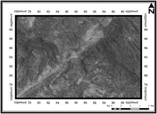
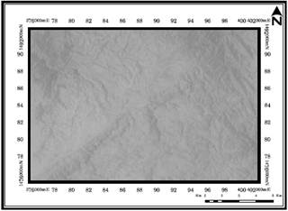
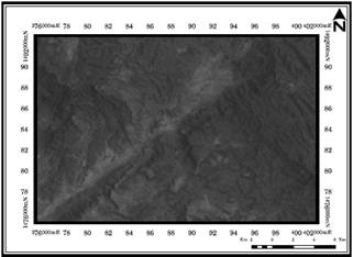
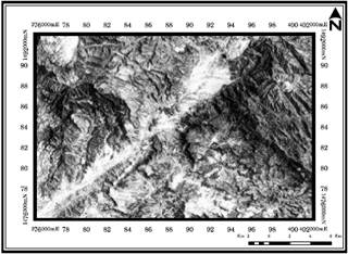
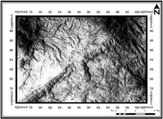
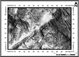
In this study,Landsat-7 (ETM) satellite image acquired on 18th Aug, 2005 with path 166 and row 51 was used. The spatial resolution of ETM is 30 m for all (three in visible, one in near infrared and two in short infrared wavelengths) while, the thermal infrared band which is 60 m, while the panchromatic image has 15 meter resolution. Based on the ability to identify features, the variance-covariance matrix, the mean and standard deviation; band 5 was selected out of a moderate (30m) spatial resolutions bands, the band 6 was used as a low (60m) spatial resolution, and the band 8 ( panchromatic) with a high (15m) spatial resolution as shown in Figs. 2,3 and 4, respectively. These selected bands were enhanced with median filter to remove the noises and rectified to be ready for other processes.
Histogram equalization can display the number of pixel values as 0 is by default displayed in black, and 255 in white, the contrast will be better when the image is displayed[23]. Histogram equalization was applied to selected bands of ETM data to obtain a high quality image visualization (Figures 5,6 and 7).
In the satellite images there is a parameter called spatial frequency which is defined as the number of changes in brightness value per unit distance for any particular part of an image. If there are very few changes in brightness value this is referred to as a low frequency, if the brightness values change dramatically over short distances, this is an area of high frequency detail [1]. Therefore, filtering operations were used to emphasize or deemphasize spatial frequency in the image. The modelling techniques in this work were achieved by several steps. The first step was to enhance and filter the different bands with different spatial resolutions using Prewitt kernel size filter in x axis and Sobel kernel size filter in y axis, the second step was to combine the two filtered images into one filtered image using SQRT function model, the third step was to create the black and white images by using binary function model, and the fourth step was to create the binary images using Delta function model. After creating binary images from different bands (bands 5,6 and 8) with different spatial resolutions, the fifth step was used to convert the points (pixels) into edges lines with colours using converting points to lines technique. The resultant images were compared with each other to find the best image which reflects all the edge lines in the area. The evaluation of these results was used to evaluate the extracted edges by overlaying the best coloured edge images with the existing fault lines from previous work (fault map), to determines where the edge lines and faults are matched. The final step was to create linear features map over the area from the best coloured edge image, then analysis and interpret the linear features based on some techniques and field data.
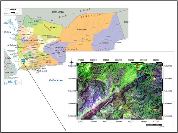
Figure 1. Location of the study area
|
|
|
| Figure 2. Original band 5 of ETM data | Figure 3. Original band 6 of ETM data |
|
|
|
| Figure 4. Original band 8 of ETM data | Figure 5. Band5of ETM with Histogram Equalization |
|
|
|
| Figure 6. Band 6 of ETM with Histogram Equalization | Figure 7. Band 8 of ETM with Histogram Equalization |
According to Sobel and Feldman [24], the Sobel operator performs spatial gradient measurement on an image and so emphasizes regions of high spatial frequency that correspond to edges. Typically it is used to find the approximate absolute gradient magnitude at each point in an input gray scale image. The operator consists of a pair of 3×3convolution kernels filters. One kernel of Sobel filter is simply by x axis, and other kernel of Sobel filter represented y axis. Mathematically, the operator uses two 3×3 kernels which were convoluted with the original image to calculate approximations of the derivatives, one for horizontal changes, and one for vertical. The Sobel filter is a method of edge detection in image processing which calculates the maximum response of a set of convolution kernels to find the local edge orientation for each pixel. If we define A as the source image, and Gx and Gy were two images which at each point contain the horizontal and vertical derivative approximations, the computations were as follows:
 (1)
(1)
![]()
![]()
![]()
![]()
In this work, the operator consists of a pair of 3×3convolution kernels filters. One kernel is Prewitt filter represented x axis and the other one is Sobel filter rotated by y axis. Prewitt filter is a method of edge detection in image processing which calculates the maximum response of a set of convolution kernels to find the local edge orientation for each pixel. This works in a very similar way to the Sobel operator but uses slightly different kernels filters [25]. The above equation (1) was modified as the follows:-
 (2)
(2)
![]()
![]()
![]()
![]()
The above equation (2) was used to filter the source images of bands 5,6 and 8 in x and y directions. The x-coordinate is here defined as increasing in the right-direction, and the y-coordinate is defined as increasing in the down-direction. At each point in the image, the resulting gradient approximations can be combined to give the gradient magnitude. Gradient magnitude may be calculated by filtering the image in two directions, horizontally and vertically, and combining the results in a vector calculation at every pixel using the following SQRT formula [25].
![]() (3)
(3)
![]()
![]()
The equation (3) was applied by SQRT equation model using ERDAS modeler to combine the x and y filtered images of bands 5, 6 and 8 of ETM data into one filtered image as shown in Figs. 8,9 and 10, respectively.
The binary equation model was used to convert the values of the pixels in the final filtered image into 0 and 1 values. Although the input data to any node can theoretically take any value, restricting it to fall within a fixed range produces more efficient values. The binary is a transformation that is devised according to each individual application to modify the input data in this manner [25]. The binary equation was used to convert the values of the pixels in the final filtered image into 0 and 1 value.
The Description of binary equation is returns true if non-zero, false if zero. The binary equation performs using the following expression:
![]() (4)
(4)
![]()
![]()
![]()
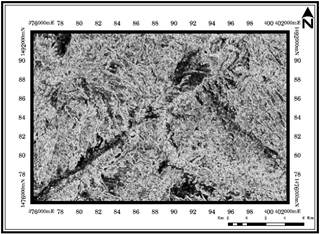
Figure 8. One filtered image produced from the band 5of ETM data by combining two filtered images after applying SQRT model
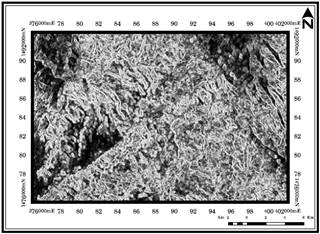
Figure 9. One filtered image produced from the band 6 of ETM data by combining two filtered images after applying SQRT model
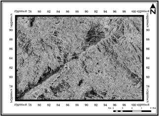
Figure 10. One filtered image produced from the band 8 of ETM data by combining two filtered images after applying SQRT model
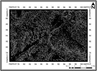
Figure 11. Black and white image with 0 and 1 pixel values produced from one filtered image of the band 5 after applying binary model
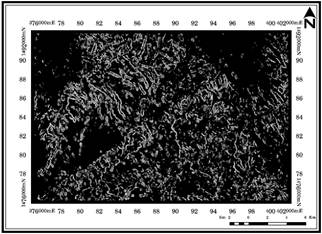
Figure 12. Black and white image with 0 and 1 pixel values produced from one filtered image of the band 6 after applying binary model
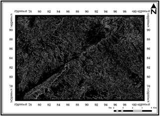
Figure 13. Black and white image with 0 and 1 pixel values produced from one filtered image of the band 8 after applying binary model
As normal, the filtered image has pixels values between 0 and 255, and applying this equation (4) was used to convert the values of the pixels between 0 and 1. By applying a binary equation model mentioned above, the original inputs were scaled to fall as continuous values between 0 and 1. The actual data sets were scaled values of pv. If the numerator less than denominator (255) the result less than one as pv goes to zero, and if the numerator equal to the denominator (255) the result equal one as pv goes to one. This means, the black colour referred to background of the image with 0 value and the white colour referred to extracted edges with 1 value .The binary equation (4) model was used to create black and white image with pixel value between 0 and 1 from filtered image using ERDAS modeler and the results of this model were shown in Figs. 11, 12 and 13, respectively.
Delta equation model was used to convert the pixels of the black colour with 0 values into same values with white colour as a image background in the binary image, and convert the pixels of the white colour with 1 values into same values with black colour as extracted edges in the binary image. The Delta can be loosely thought of as a function on the real line which is zero everywhere except at the origin, where it is infinite. As a formal definition by Richards and Jia [26], the best that can be done was:
![]() (5)
(5)
![]()
![]()
![]()
In this paper, the Delta function was modified to be suitable with the modelling in this work as follows:
![]() (6)
(6)
![]()
![]()
The equation (6) was applied using Delta equation model within ERDAS modeler to convert the pixel values and colour of the black and white images of band 5,6 and 8 into binary images. The results of this model were shown in Figs. 14, 15 and 16, respectively.
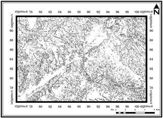
Figure 14. Binary image produced from the black and white image of the band 5 after applying Delta model
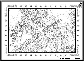
Figure 15. Binary image produced from the black and white image of the band 6 after applying Delta model
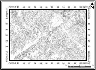
Figure 16. Binary image produced from the black and white image of the band 8 after applying Delta model
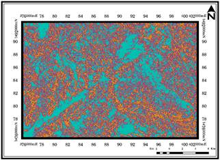
Figure 17. Coloured edge image produced from binary image of the band 5. Edges represented by dark golden yellow colour and background represented by cyan colour
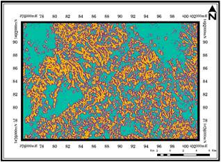
Figure 18. Coloured edge image produced from binary image of the band 6. Edges represented by golden yellow colour and background represented by cyan colour
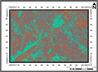
Figure 19. Coloured edge image produced from binary image of the band 8. Edges represented by dark yellow colour and background represented by greenish cyan colour
The final step of this modelling technique was the convert model. This model used to convert the binary images produced from bands 5,6 and 8 into coloured edge images as shown in Figs. 17,18 and 19 respectively. The converting technique was used in this study based on the pixel to line convert model within PCI geomatica modeler (version 9.1), while the edges can be appeared as lines within resultant maps. Hence, the edge lines will be easy to recognize and interpret as linear features occurred in the area.
The evaluation of three coloured edge images was used using overlaying capability technique with help of the fault map of the study area to determine the best coloured image based on the extracted edges and fault lines were matched. The fault map of the study area was digitized from pervious works of Taiz geological sheet map with scale 1:250,000 produced by Geological Survey of Yemen [27], as shown in Fig. 20.
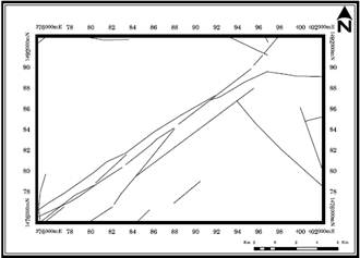
Figure 20. The fault map of the study area (Source: GSY ,1990)
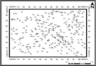
Figure 21. Locations of the strike/dip reading of the fractures collected from the field
269 reading of structural data such as joints, fissures and fractures were collected during the field work stations (Figure 21). These data were used for structural analysis of linear features of the area. Rose diagrams of linear features, fault lines and fractures measured in the field were created using Rockworks software 2006 to determine the major trend directions of the structural features in the area. Moreover, stereonet program within Rockworks software was used to analysis the fractures data collected from the field. These data were strike/dip reading of fractures like joints and fissures. The structural analysis of these fractures gives an idea about the direction of principal stress deformation in the investigated area. The structural readings were plotted as points (pole to plane) represented by contour densities tend to line up along a great circle. This analysis was used to find the principal stress direction of deformation (tensional deformation) in the study area.
3. Results and Discussions
The modelling technique mentioned above were used with ERDAS modeler for creating binary images over the study area showing the edge detected from bands 5,6, and 8 of ETM data, respectively. The range of histogram intensity from 0 to 255 was used in this enhancement which equal to 100% of threshold value for the entire three bands enhancement. Image enhancements were used to improve the appearance of an image and make it easier for visual and/or automatic analysis and interpretations of imagery. Careful inspection of Landsat ETM images demonstrates that the drainage lines (network) were clearly observed bands and could be extracted in the binary image. The drainage lines were considered as edges.
Based on the visual interpretation, the relationship between pixel distribution and edge appearance of the three binary images (Figures 14,15 and 16) was observed. The binary image produced from the band 5 shows a good relation between pixel distribution and edges, while the edges were quite good appeared and easy to recognized. Binary images extracted from the bands 8 and 6 show a poor relation between pixel distribution and edge appearance. The results show that, the number of black pixels (465255) in the binary image of the band 5 more than the number of black pixels (124137) in the binary image of the band 6 and less than the number of black pixels (1987425) in the binary image of the band 8. Moreover the edges extracted from the band 5 were much cleared, and reflect most of the edges in the original image. On the contrary, the result of edges extracted from the band 8 not very cleared and more complexes, as well the band 6 shows very less edges compared with the bands 5 and 8, respectively.
The detection of the pixels(edges)of the binary image created from high resolution (band 8) was more than the pixels (edges) obtained by other binary images produced from bands 5 and 6, respectively. The edges detected from the binary image with a high (15m) resolution show huge black pixels of edges, thus, showing more complex edge image. This relationship is possibly due to the fact that the binary image from high resolution approaches do not discriminate edge features during the analysis, and this leads to increasing the number of the pixels which reflect the edges. This explains possibly why the number of the pixels obtained from a moderate and low resolution images was less. On contrary, edges detected form the binary image of the band 6 was less compared with other results. This is because of spatial resolution of this band.
Meanwhile, image enhancements with edge modelling technique were used to improve the appearance of edges in the images and make it easier for visual and/or automatic analysis and interpretations of imagery. The using of different image resolutions for edge detection based on the logarithm functions within edge modelling technique followed by results comparison yields more effective results in term of visual interpretation. The results of these modelling show that, the moderated 30m resolution of ETM data was proved to be better for edge detection compared to the low and high band resolutions of the same data. Therefore the spatial resolution such as a high spatial resolution and low spatial resolution could not be useful for edge detection (edge lines).
Three binary images produced from the bands 5,6 and 8, were converted into coloured edge images as shown in Figs. 17,18 and 19, respectively. The converting technique was made in this study to convert the pixels of edges into edge lines. Hence, the edge lines more easily to recognize analysis and interpret. The visual interpretation with help of DEM, drainage pattern and fault maps of the area was made based on continuous edge lines appearance in the coloured edge image to be easy for interpretation. Generally, visual interpretation of the results (coloured edge images) shows that, the coloured edge image produced from the binary image of the band 5 was a better image for appearance of edge lines compared with other images. For this reason, the coloured edge image produced from the binary image of the band 5 was considered in this study for linear features mapping.
4. Results Evaluation
For more evaluation, coloured edge images were tested for their accuracy with the help of fault lines of the fault map using overlaying technique that determines where the edge lines and fault lines are matched. Then, calculate the edge lines - fault lines matching percentage to get the best coloured edges image produced over the study area.
For this purpose, the re-sampling technique was applied in this work to resample the resolution of the fault lines map as same as the resolutions of the coloured edge images. Moreover, three fault lines maps with 30m, 60m and 15m resolutions were generated as well, a buffer zone of 30m,60m and15m was assigned to the fault lines of fault maps with 30m, 60m and 15m resolutions, respectively. Then, the resultant fault maps matched with the coloured edge images with 30m, 60m and 15m resolutions, respectively.
The total matching percentage between the fault lines and edge lines was calculated to be 75.69% for the image produced from the band 5 with a moderate (30m) resolution, 58.6%for the image produced from the band 8 with 15m resolution and 32.5% for the image produced from the band 6 with 60m resolution. The results of matching techniques between fault lines and the edges lines of the band 6 with a low (60m)spatial resolution of and the band 8 with a high (15m)spatial resolution show that, there were no good relationships between edges and faults lines. For this reason, these images were not considered. But the edges of band 8 could reflect the small linear features in the study area. However, the result of matching between edges of a moderate (30m)spatial resolution of the band 5 seems to be the best result of matching technique in this study. It is clearly seen that, most of the fault lines were exactly matched with edge lines. The most important feature in the area is the presence of edge lines patterns and reflect the fault zones system in the center of the area. It is concluded that, there is a good relationship between these edges and fault lines. The moderate (30m) resolution was yield more effective results and was taken into consideration.
5. Linear Features Extraction
The faults were believed to be disconnected because of geological processes or because of an unclear image. In accordance with that assumption, there are many edge lines could be found in the best coloured edge image of the band 5 may reflect the same shape and pattern of the edge lines that match true fault lines. Moreover, these edge lines were not matched with the fault lines may reflect the new fault lines within this area which not previously mapped.
The visual interpretation of the shape and pattern of edge lines from the best coloured edge image with helps of a topographic map, a drainage pattern map, and three dimensions of DEM, the new fault lines could be recognized from the best coloured edge image. These edge lines were drawn as segment lines, considering these lines as new faults may occurred in the area.
The 114 segment lines were mapped in the area represented by black colour lines, whereas, 27 true fault segments (previously mapped) also mapped represented by blue colour (Figure 22). The minimum length of linear features was controlled in length to be more than 1 km within the final linear features map. Hence, linear features in length of 1 km and more are interpreted to represent faults. Based on the pattern of these segments(except the segments of true fault lines), there are 34 fault lines may occur as new faults in the study area and it should be taken into consideration.
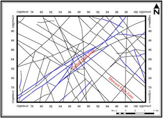
Figure 22. Linear features map extracted from coloured edge image of the band 5, the new fault segments represented by black colour lines, the true fault segments (previously mapped) represented by blue colour lines and the names of fault zones also included
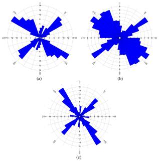
Figure 23. Rose diagrams show the NW-SE and NE-SW as the major trend directions of the structural linear features in the study area. a- rose diagram of linear features, b-rose diagram fault lines of the whole Taiz area, and c- rose diagram fractures measured in the field
To determine the azimuth orientations of structural linear features in the area, rose diagrams was prepared for linear features, fault lines and fractures measured in the field (Figure 23). These diagrams show the NW-SE and NE-SW are major dominant trends of the structural linear features in the study area, while the N-S and E-W are minor dominant trends.
Based on the pattern of the linear features and/or edges, the length, and spatial distributions, trend analysis of linear features and field observations, there are two fault systems could be occurred in the study area. The first fault system with NW-SE trend set direction was predominant and the second fault system shows the NE-SW trend set direction (Figure 22). Moreover, the faults with N-S and E-W trend set directions also observed.
Structural analysis of the fractures measured in the field was made using best fit great circle technique of a stereonet program within rockworks software (Figure 24). The result of this analysis shows the NW-SE was the tensional force direction of the deformation acted in the area. Based on this analysis, the first NW-SE and second NE-SW sets of linear features are sets of normal and reverse faults, and the third E-W and fourth N-S sets of linear features are sets of shear fractures (strike slip faults). This force of deformation was acted in the study area may resulted from the activation of the Opening Red Sea Rifting Zone.
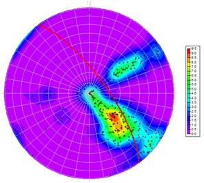
Figure 24. Astereonet graph showing the reading concentration of fractures measured in the field and the best fit great circle represented by red colour as NW-SE direction of deformation
The linear features map and field observations suggest that, there are two fault zones were observed in the area. The names of these fault zones were given in this research as Mawasit and Turbah Fault Zones. The Mawasit Fault Zone located in the south-east part of the area with the NW-SE strike direction and NW dip direction. This fault zone was not mapped and known from literature. The NW-SE strike direction of the Mawasit Fault Zone appeared to be parallel to the trend of the Opening Red Sea Rifting System. Therefore, there is a relationship between this rifting system and the occurrence of this fault zone. The Turbah Fault Zone well defined zone in the central part of the area with the NE-SW strike direction and SE dip direction. This fault zone was mapped and not well known from literature. The NE-SW strike direction of the Turbah Fault Zone appeared to be parallel to the trend of the Gulf of Aden Rifting System. Therefore, there is a relationship between this rifting system and the occurrence of this fault zone.
6. Conclusion
In this study, decreasing the cost and increasing the efficiency of detecting edges sets with different pixel resolutions using logarithm functions with building models for edges extraction yields more effective results. Based on visual interpretation and overlying technique, the band 5 of Landsat-7 Enhanced Thematic Mapper (ETM) with a moderate resolution (30m) appeared to be better source of the spatial edge variations compared with a high (15m) and a low (60m) pixel resolutions bands. However, the detected edge from a high (15m) spatial resolution of the band 8, mostly resemble a short fracture lines may occur in the study area. The application of edge modelling technique including integrated different filters, SQRT, Delta and convert models is an excellent tool to extracted and understand variation of edges by visual and/or automatic interpretation. In this study, 34 linear features were extracted from the coloured edge image of band 5 identify as new fault lines in the area. The mean trends observed from the linear features map, geological map of whole Taiz area and fractures measured in the field were NW-SE and NE-SW as the major trends of the structural linear features in the area. The structural analysis of the fractures measured in the field was used to find the principal direction of deformation acted in the area as well to classify the linear features. Based on joints and fissures (fractures) analysis, the direction of the tensional direction of deformation can be estimated as NW-SE. The system of linear fractures in the study area consists of four major sets. The first NW-SE and second NE-SW direction sets of linear features are sets of normal and reverse faults, respectively and the third E-W and fourth N-S direction sets of linear features are sets of shear fractures (strike slip faults). There were two fault zones were observed in the study area, such as the Mawasit Fault Zone well developed in the south-east part of the area with NW-SE strike and NW dip directions and parallel to the trend of the Gulf of Aden Active Rifting System, whereas, the Turbah Fault Zone located in the central part of the area with NE-SW strike and SE dip directions parallel to the trend of the Opening Red Sea Rifting System. These faults formed as a result of active rifting systems effects. Meanwhile, any methods can be used to enhance the edges in any image, but extract these edges by using edge models leads to updating and revising existing geological maps in the study area.
Acknowledgment
Authors would like to thank all staff in the Geology Department, Faculty of Applied Science, Taiz University, Taiz, Yemen, for their support to this research.
References
- Leica Geosystems. (1999). Erdas Imagine 8.5. ERDAS Field Guide. 5th edition. USA: Atlanta: Georgia, Inc.
- Jensen J R. (1996). Introductory Digital Image Processing: a remote sensing perspective. 2nd edition. U.S.A: Prentice Hall Inc.
- Koike K, Nagano S, Ohmi M. (1995). Lineament Analysis of Satellite Images Using a Segment Tracing Algorithm (STA). Computers & Geosciences, 21 (9), 1091-1104.
- Jordan G, Schott B. (2005). Application of Wavelet Analysis to the Study of Spatial Pattern of Morphotectonic Lineaments in Digital Terrain Models. A case study. Remote Sensing of the Environment 94: 31-38.
- Gupta R P. (1991).Remote Sensing Geology. Berlin, Heidelberg: Springer-Verlag.
- Shorth N M. (2004). Lineaments and Fractures. Remote Sensing Tutorial. http://rst.gsfc.nasa.gov/Sect2/Sect2_8.html. Accessed November 24, 2007.
- NASA. (2005). The Remote Sensing Tutorial. Section 1: Image Processing and Interpretation - Morro Bay, California as the Test Image. Spatial filtering. http://rst.gsfc.nasa.gov. Accessed June 25, 2008.
- Arlegui LE , Soriano MA. (1998). Characterizing lineaments from satellite image and filed studies in the central Ebro basin ( NE Spain). International Journal of Remote Sensing. 19 (16): 3169-3185.
- Masoud A, Koike K. (2006). Tectonic architecture through Landsat-7 ETM+/ SRTM DEM- derived lineaments and relationship to the hydrogeologic setting in Siwa region, NW Egypt.Journal of African Earth Sciences. 45: 467-477.
- Mah A, Taylor GR, Lennox P, Balia L.( 1995). Lineament Analysis of Landsat TM Images, Northern Territory, Australia. Photogrammetric Engineering and Remote Sensing. 61(6): 761-773.
- Minor T B, Carter J A, Chesley M M, Knowles R B. (1994). An integrated approach to groundwater exploration in developing countries using GIS and remote sensing. Proceedings of the International American Congress on Surveying and Mapping. American Society for Photogrammetry and Remote Sensing. (ACSM/ASPRS) 418-428.
- Casas A, Cortes M, Angel L, Maestro A, Soriano, M A, Riaguas A, Bernal J. (2000). A program for lineament length and density analysis. Computers and Geosciences. 26(9-10), 1011-1022.
- Koike K, Nagano S, Kawaba K. (1998). Construction and analysis of interpreted fracture planes through combination of satellite-image derived lineaments and digital elevation model data. Computers & Geosciences. 24: 573-583.
- Mavrantza O D, Argialas D P. (2003). Implementation and evaluation of spatial filtering and edge detection techniques for lineament mapping – Case study : Alevrada, Center Greece. Proceeding of SPIE International conference on remote sensing. remote sensing for Environment Monitoring, GIS Application, and Geology II. Edited by Ehlers, M. SPIE 4886: 428-717.
- Wang J, Howarth P J. (1990). Use of the Hough Transform in Automated Lineament Detection. IEEE Transactions on Geoscience and Remote Sensing. 28( 4): 561-566.
- Abdullah A, Akhir M J, Abdullah I. (2010). Automatic mapping of lineaments using shaded relief images derived from digital elevation model (DEMs) in the Maran-Sungi Lembing area, Malaysia. Electronic Journal of Geotechnical Engineering. 15: 949–957.
- Abullah A, Nassr S, Ghaleeb A. (2013).Landsat ETM-7 for Lineament Mapping using Automatic Extraction Technique in the SW part of Taiz area, Yemen. Global Journals Inc. (USA). 13 :49-52.
- Abdullah A, Akhir M J, Abdullah I. (2009). A comparison of landsat TM and SPOT data for lineament mapping in Hulu Lepar area, Pahang, Malaysia. European Journal of Scientific Research. 34: 406–415.
- Abdullah A, Akhir M J, Abdullah I. (2010). The extraction of lineaments using slope image derived from digital elevation model: case study of Sungai Lembing-Maran area, Malaysia. Journal of Applied Sciences Research. 6:1745–1751.
- Abullah A, Nassr S, Ghaleeb A. (2013).Remote Sensing and Geographic Information System for Fault Segments Mapping a Study from Taiz Area, Yemen. Journal of Geological Research. 2013: 16 . http://dx.doi.org/10.1155/2013/201757.
- Kocal A, Duzgun HSB, Karpuz C. (2004). Discontinuity Mapping with Automatic Lineament Extraction from High Resolution Satellite Imagery. Proceedings of 20th Congress of International Society for Photogrammetry and Remote Sensing (ISPRS) 37:1073-1078.
- Cortes AL, Soriano M A, Maestros A, Casas AM. (2003) The role of tectonic inheritance in the development of recent fracture systems, Duero Basin, Spain. International Journal of Remote Sensing, 24: 4325-4345.
- Gonzalez R, Woods R. (1992). Digital Image Processing. Addison-Wesley Publishing Company.
- Sobel I, Feldman G. (1968). A 3x3 Isotropic Gradient Operator for Image Processing, presented at a talk at the Stanford Artificial Project in 1968, unpublished but often cited, orig. in Pattern Classification and Scene Analysis. Duda,R. & Hart,P. John Wiley & Sons. 73:271-272.
- Schowengerdt R A. (2007). Remote Sensing: Models and Methods for Image Processing. 3rdedition. New York: Elsevier Academic Press. Inc.
- Richards J A, Jia X. (2006). Remote sensing digital image analysis: An introduction. 4th edition. Berlin, Heidelberg: Springer. Verlag.
- Geological Survey of Yemen (GSY).( 1990).Geological Map of Taiz Area. Scale 1:250, 000.


