Remote Sensing Study of Land Use/Cover Change in West Africa

Addo Koranteng^{1, *}, Tomasz Zawila-Niedzwiecki², Isaac Adu-Poku³

¹Institute of Research Innovation and Development (IRID), Kumasi Polytechnic, Kumasi, Ghana

²Faculty of Forestry, Warsaw University of Life Sciences, Warsaw, Poland

³Rudan Engineering Limited, Accra, Ghana

Abstract

Increasing population and other anthropogenic activities have profound effect on large areas of forested land and other land use/cover forms throughout the world. There is a certain cause and effect relationship between changing practice for development and land use change, thus necessitating an assessment of land use dynamics and the projection trend. A combination of geospatial and remote techniques were utilized to evaluate the present and future landuse/ landcover scenario of southern part of the Western Region of Ghana. Multi-temporal satellite imageries of the Landsat series and DMC were used to map the changes in land use from 1990 to 2010. Four major land use classes (Forest, Agriculture, Built-up and water) were considered as the most dynamic land cover/use (LULC) practice. Markov modelling was applied for prediction of probable land use/ land cover change scenario for the years 2020, 2030 and 2040. The study showed that in years 2020 to 2040 in the predictable future, there will be a gradual increase in built up areas, while a stability in agricultural land use is envisaged. Agricultural land use would still remain the dominant land use type. Forests would be drastically reduced from close to 87% in 1990 to just fewer than 20% in 2040. This precarious situation would demand that prudent land use decisions to be made to keep Ghana’s REDD+ program on track and to mitigate the effects of the climate change phenomenon.

Keywords

Land Use Land Cover, Cellular-Automata-Markov, Land Use/Cover Modelling, Remote Sensing

Received: September 7, 2016
Accepted: September 18, 2016
Published online: October 19, 2016

@ 2016 The Authors. Published by American Institute of Science. This Open Access article is under the CC BY license. http://creativecommons.org/licenses/by/4.0/

1. Introduction

Land cover alterations have profound effects on biotic and abiotic components in the earth’s ecosystems’ ([10]; [17]; [29]; [30]. Mankind habitation on earth and its associated activities have resulted in many alteration of the landscape which has had adverse effect on the natural environment. These anthropogenic effects on the environment are reckoned as key drivers of environmental change [32]. Land-use and land-cover change emanates from the complex interaction of a vast number of both natural and manmade factors [9]; [8]. Changes in land cover are prevalent, progressively rapid, and have adversative impacts and implications at local, regional and global scales. The dynamic factors and mode of change in land use /land cover (LULC) are vital for studying the environment and subsequent effects [39]. [37] advances that, precise mapping of LULC and its modifications are pivotal to land use studies the world over.

Remote sensing gives the opportunity for fast data acquisition of land use data at relatively lower cost than ground survey methods and offer time series data of LULC, which are suitable to ascertain the spatio-temporal modifications and its probable effect on the environment.

Fuel wood gathering for firewood and charcoal making, and livestock grazing (to a lesser extent) in forests are deemed as the most significant drivers of forest degradation in Africa. The fundamental causes are the complex mix of economic, social, political, cultural and technological processes that impact on the direct drivers (logging, mining, agriculture and expanding human settlements) of deforestation and forest degradation [1]; [5]; [14]; [19]. These direct drivers impact at several levels such as local conditions (subsistence livelihood, poverty and culture); at national levels (population growth, domestic markets, state policies, legislations and laws) and at the international level (world markets demands, commodity prices for goods and services). [15] add that, economic development which is chiefly dependent on the export of primary commodities (raw materials) and the world’s large market for timber and other agricultural produce are the indirect drivers of deforestation and degradation.

Land use and land cover change (LUCC) has been acknowledged as chief drivers of environmental change at all spatial and temporal levels [22]. Accurate and up-to-date land cover change information is necessary to understanding and assessing the environmental consequences of such changes [11]. [34] defines change detection as the method of identifying changes in the state of an object or phenomenon by observing it at varying times. Change detection is an indispensable process in the observation and management of natural resources. It helps urban development planning as it gives quantitative analysis of spatial distribution which is of population of interest. Change detection is valuable in many applications such as disaster monitoring, deforestation and afforestation assessments, tracking shifting cultivation practices, a land use change analysis, vegetation phenology changes, seasonal changes in pasture production, damage assessment, crop stress detection,, and other environmental phenomenon.

There are wide ranging approaches in predicting Land-Use, Land-Use Cover, and Forestry (LULUCF). These approaches vary based on purposes, methodologies, geographic areas of the analysis, assumptions and both the source and type of data employed. Geographic/ Land-Cover, Economic/land-use change and Model Linkages and Integration are examples models [21]. Geographic/land-cover models have been enhanced by the quick development of remote sensing and Geographic Information Systems (GIS). Spatial measurement and geographical/physical features of the land problem are dominant to this category of analysis.

Markov chain analysis has been employed as an effective tool in modeling and forecasting land cover change [16]. A Markov chain is a discrete random process with the property that the future state of system at time t2 can be modelled solely on the basis of the current state at time t1 [6]. Accordingly, the knowledge of a current state of system offers ample information on the future state and does not hinge on the history before the current state at time t1. The Markov chain process uses two classified images to generate a transition probability matrix which represents the conditional probability for a transition from one class at time t1 to another at time t2. The accuracy of the predicted land cover map is based on the accuracy of the individual classified images. This model is used to forecast changes in LULC in different spatial scales. Cellular Automata-Markov has been used for LULC modelling studies; [16] used Cellular Automata-Markov to assess land use change in the lower half of the Ashanti Region of Ghana within a 40 year period 1990-2030. [31] perused land use and land cover changes in Kermanshah City, Iran from 1987 through 2000 to 2006.

Markov chain model was precisely chosen for this study because it is relatively simple to use and gives satisfactory results.

This study focuses on identifying the conversion of forests into other land use forms in Western Region. The study again examines the stochastic nature of the LULC and predicts change in the future.

2. Methodology

2.1. Study Area

Ghana is located along the west coast of Africa and covers about 23 million hectares. It is bounded by the Ivory Coast to the west, Burkina Faso to the north and Togo to the east and the Gulf of Guinea (part of the Atlantic Ocean) to the south (Figure 1). It lies between latitude 4° 45′ and 11° 11′ north and extends from longitude 1° 14′ east to 3° 17′ west.

The Western Region occupies an area of 2,391 km², which is approximately 10% of Ghana’s land size. 75% of its vegetation is within the high forest zone of Ghana. Rain forest intermingled with patches of mangrove forest along the coast and coastal wetlands are found in the south-western areas of the region. High tropical forest and semi-deciduous forest are situated in the northern part of the region. 24 forest reserves, which represent about 40% of the forest reserves in Ghana, are located here. The Western Region is the largest producer of Ghana’s two premium plant exports products, cocoa and timber. It has large quantities of gold and bauxite as well [43].

The Area of study (AOI) has the following administrative districts Aowin-Suaman, Jomoro, Nzema East and Wasa Amenfi all in the Western Region of Ghana and endowed with the following protected forests and wild life reserves Yoyo, Sui River, Tano Ehuro, Tano Anwia, Bion River, Jema Assamkwa, Boi Tano, Fure

Headworks, Tano Nimiri, Mamiri, and Buru River.

2.2. Materials

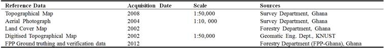
Satellite images (Landsat TM, Landsat ETM+ and Disaster Monitoring Constellation-DMC)-Table 1 and Reference data (Table 2) were acquired from the Forestry Commission of Ghana, under the Forest Preservation Program (FPP-Ghana) 2011/2012.

Table 1. Remote Sensing Images.

Table 2. Reference data.

2.3. Image Processing

Pre-processing processes such as geometric corrections, radiometric corrections, subset creation and image enhancement on the images before classification.

Geometric Corrections: For both the Landsat TM Bands 1, 2, 3, 4, 5 and 7 were stacked together. Band 6 which measures thermal reflectance was not included because of its different spatial resolution of 120m and moreover the study was not measuring heat reflectance. The resultant stacked images which were in the global coordinate system, UTM WGS 84 were re-projected onto the Ghana datum, War Office which is based on Traverse Mercator Projection. All the images (Landsat TM, Landsat ETM+ and DMC) were re-sampled to 30 x 30 meter pixel resolution to make accurate analysis of the datasets and comparability possible.

Radiometric Corrections: Radiometric calibration was carried out on satellite imageries prior to image classification and generation of spectral indices. Datasets were already corrected to some extent; but the 1989TM, and 2000ETM+ images were quite hazy and therefore corrected.

ERDAS Imagine 9.1 was used to undertake the image processing and Land use/cover Classification. Idrisi 17.0 Selva Edition was used to handle the for the Change detection and projection part of the study. ARCGIS 10.0 was employed to produce the output maps, while Microsoft Excel was used to produce the graphs.

2.4. Land Use Classes

The following broad land use/cover classes were chosen based on satellite image availability and study of literature.

Agriculture: This consist of cropped land, including rice fields, and plantation where the vegetation structure falls below the thresholds used for the Forest Land category. Land where over 50% of any defined area is used for agriculture, this may be currently cropped or in fallow and may include areas for grazing of livestock.

Built-Ups: These specify all developed land, including social utilities such as transportation infrastructure (roads and highways), built up areas, bare grounds and human settlements of any size.

Forest: This includes all land with woody vegetation consistent with measurements used to outline Forests in the national greenhouse gas inventory. Additionally all vegetation structure that currently fall below, but in situ could potentially reach the Ghana’s threshold values. Minimum Mapping Unit (MMU) is 1.0 ha; Minimum crown cover is 15%; Potential to reach minimum height at maturity (in situ) as 5 meter

Water: These include lands that are covered or saturated by water for all or part of the year (for example peatlands). It also includes reservoirs and natural rivers and lakes.

2.5. Image Classification and Land Cover Map Generation

The satellite imageries of 1990, 2000 and 2010 were transformed into thematic land cover using supervised classification by Maximum Likelihood Classifier (MLC) and spectral indices based thresholding of corrected satellite imageries. As the study mainly concentrates on the analysis of vegetation cover change, first level classification was performed and four major land cover classes (Agriculture, Built ups, Forests and Water) were considered. The training sets were collected from the field using handheld GPS. Sixty (60) training sets signifying the different land use/cover classes (Forest-12, Agriculture-28, Built-Ups-16 and Water-4) were digitized on the individual epoch images (1990 TM, 2000 ETM+ and 2010 DMC) using the AOI tool and named consequently in the signature editor of ERDAS imagine 9.1 and Supervised Classification\ undertaken.

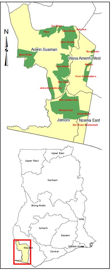
Figure 1. Western Region Study Area.

The 60 classes ensuing from the 60 training areas were recoded into the broad classes (Forest, Agriculture, Built-Ups and Water) via of the Image Interpreter/GIS Analysis/Recode tool in ERDAS Imagine 9.1. The 12 forest classes were recoded as one assigned the color deep green, the 28 Agriculture Classes recoded as Class two and given color yellow; the 16 Built-Ups classes recoded as three and set as Maroon and the 4 classes of water recoded as 4 and apportioned color blue.

The classified imageries for 1990, 2000 and 2010 were validated using error matrix and Kappa statistics. Error matrix is as one of the common techniques for measuring the accuracy of thematic map [35]. It measures a sample from a particular category of the classified map and the actual category can be verified from the ground or reference data [4]. Reference data extracted from table 2 were used to perform Accuracy Assessment. This study evaluated the accuracy of the classified images from the matrix generated. Calculation of areas in hectares of the resulting land cover types for each study year was carried out subsequently.

2.6. Markov Chain Modeling

Markov chain model evaluates two qualitative land cover images of different dates [23] and yields a transition probability matrix, a transition area matrix, and a set of conditional probability images [12]; [38]. The probability that each land cover category will change to every other class is called the transition matrix. Transition areas matrix records the number of pixels that are expected to change from each land cover category to other land cover type over the definite number of time units. The model also provides a set of conditional probability images for each land cover category. These maps express the probability that each pixel will belong to the designated class in the next time period. They are called conditional probability maps, since this probability is conditional on their current state. Given the set of conditional probability images produce any number of potential realizations of the projected changes embodied in the conditional probability maps. To improve the spatial sense of these conditional probability images using redistribute of the statistic such that it follows the suggested pattern, but maintains the overall area total. In the Markov chain model, usually, land cover change is considered to be a stochastic process and diverse classes are considered in the states of a chain.

Two land cover maps 1990 and 2000 were first employed to predict the land cover map of 2010. This predicted 2010 land cover map was compared with the actual land use/cover map of 2010 produced in ERDAS Imagine for validation. After the successful validation, the 1990 and 2000 land cover maps were again used to predict land use/cover map for the years 2020, 2030 and 2040.

3. Results

The results are described in five sections; Study area delineation, land use / land cover classification, Accuracy Assessment, Change detection and land use/cover prediction.

Figure 2. AOI Landsat TM 1990.

Figure 3. AOI Landsat TM 2000.

Figure 4. AOI DMC 2010.

3.1. Study Area Delineation

The supervised classification employed in this study produced three land use/cover maps from the three multi-temporal images – 1990TM, 2000 ETM+ and 2010 DMC. The Study Area was categorized into four main land use/cover classes as described in section 2.4. The resultant land cover maps are shown in figures 6, 7 and 8. Table 3 displays the extent of the area of the individual land cover categories in hectares (ha) and the percentage they occupied.

The land use/cover map for 1990 (figure 5) forest constitutes almost 90% of the total LU. Agriculture is just 10% and Built up at around 4%. Water is under 1%.

The land use/cover map for 2000 (figure 6) Forest is still the dominant LU type but has lost more than 30%. Agriculture LU has appreciated from 10% in 1990 to 40%. There is marginal increase in Built-up to around 4% from 3% in 1990. Water share remains under 1%.

The land use/cover map for 2010 (figure 7) Agriculture assumes the dominant LU at almost 70%, forest share now at stands at 27% from 56% in 2000. Built-up adds another 1% to make it 4%. Water share remains the same.

Table 3. Area of categories in Hectares -Western Region.

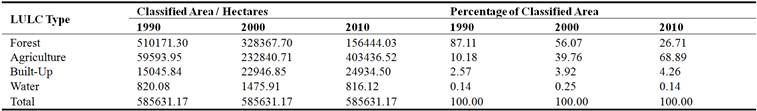
Figure 5. LULC 1990 Map.

Figure 6. LULC 1990 Map.

Figure 7. LULC 1990 Map.

3.2. Accuracy Assessment

Accuracy assessment undertaken on the 2010 DMC image classification and an assessment report was generated in an error matrix, and a Kappa statistics. An overall classification accuracy of 79.17% and 0.6516 as the overall Kappa statistics were achieved. Accuracy assessments for 1990 epoch TM and 2000 epoch ETM+ images accuracy results were 78.42%; 0.6404 (1990 epoch TM) and 80.12%; 0.7076 (2000 epoch ETM+) for Classification accuracy and Kappa Statistic respectively.

3.3. Change Detection 1990 - 2010

The table 4 displays the extent change of the area of the individual land cover categories in hectares (ha) and the percentage they occupied for 1990-2000 and 2000-2010.

Figure 8 indicates the changes that have transpired for the period 1990 – 2000. An area of 223536.50 ha representing 38% of the study area of 585631.17 ha had undergone change. The largest change was noticed as forests were converted to agriculture at 87%. A marginal gain forest gain was recorded as agricultural land had also been converted in Forests at 10%. Agricultural land gave way to Settlement at 1.56%, while forests were converted to Built-ups 10%.

Table 4. Change detection 1990-2000 and 2000-2010 for Western Region.

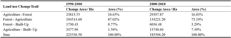
Figure 8. Change Trajectory 1990-2000.

Figure 9 show the variations that have occurred between 2000 and 2010. Forested land gave way to agriculture at 73% reckoned as the biggest change. Agricultural land was converted into forested land was reckoned as the second biggest change at less than 16%. Forest lost out to Built-Ups at less than 4%. Agriculture gave way to Built-Up at 7%.

Figure 9. Change Trajectory 2000-2010.

The LCM model in Idrisi generated from 1990 – 2000 and 2000 - 2010 change trajectory maps are shown in Figures 10 and 11. The figures reveal the degree of changes (Gains + and Losses) in the study area resulting from the land cover conversions. It can be deduced that with the exception of water all other land cover classes experienced some form of transition either gain or loss. Forests lost out heavily mostly to Agriculture and Built-Ups gained from Agriculture mostly and from Forests. These revealed that, forest loss was extensive.

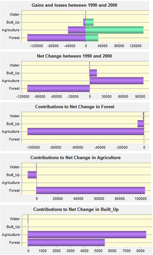
Figure 10. Trend Analysis 1990-2000.

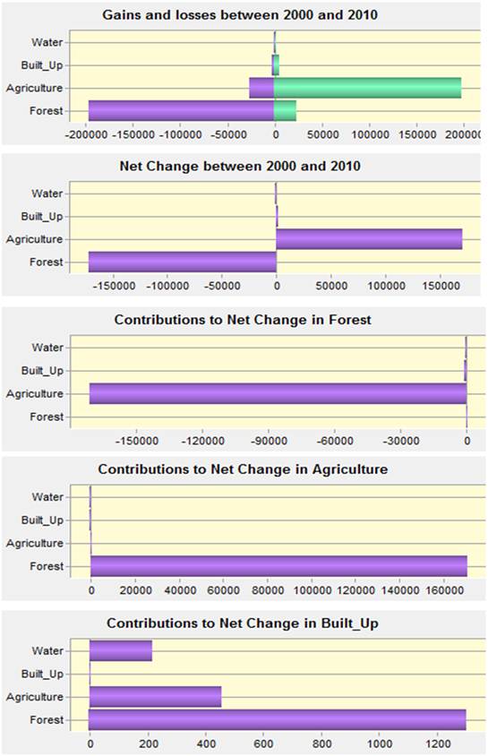
Figure 11. Trend Analysis 2000-2010.

3.4. Land Use/Cover Prediction

Markov Chain Analysis was employed to forecast the future land use/cover map for year 2010 using the land use/cover maps of the years 1990 – 2000. This projected map was then compared with the actual land cover map of 2010 for validation (Figure 12). Validation is reckoned to play a vital role in the modeling process. A validation process was undertaken to ascertain how well the predicted map resembled the reference map. The validation used kappa statistic generated from VALIDATE module in Idrisi. The Kno indicates the overall accuracy of prediction at 79.25%. Other kappa statistics like Klocation and Kquality were computed to be 74.20% each. These values are within the standard values suggested by [24] explains that a value of kappa of 75% or greater show a very good to excellent classifier performance, while a value less than 40% is poor.

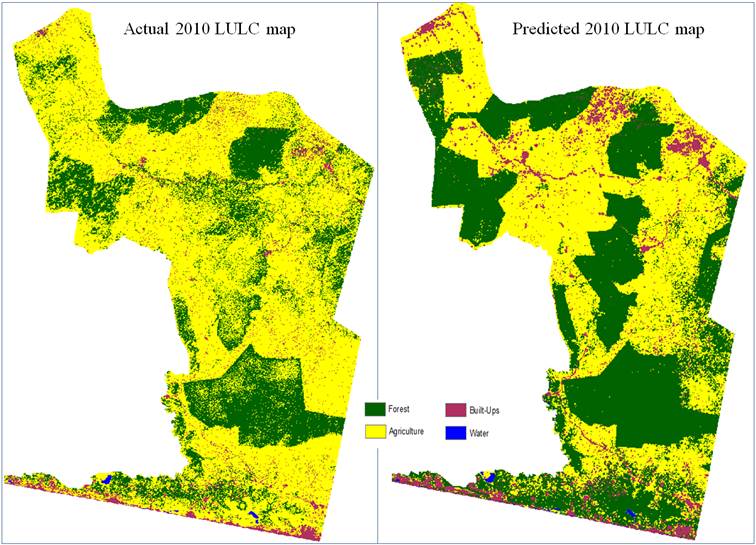
Figure 12. 2010 Validation (Actual & Predicted).

Table 5. Predicted Land use/cover for 2020, 2030 and 2040 in the Western Region.

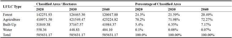
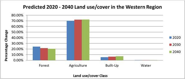
Figure 13. Land use/cover trend 2020-2040.

Table 5 displays the predicted extent of the area of the individual land cover categories in hectares (ha) and the percentage they occupied and Figure 13 indicates the graph depicting the trends of land cover changes in the years 2020 and 2040.

Figure 14 displays the predicted 2020 land use/cover map. Forest cover would be cut to 24%. Agriculture would continue to lead at the expense forest cover. Built-Up category would increase marginally at the expense of Agriculture. Water level will reduce marginally as well.

Figure 15 shows the predicted 2030 land use/cover map. Forest cover would decrease further to 22%. Agriculture would appreciate and would be the dominant land use class taking from the forest cover. Built-Up category would increase slightly to 6%. Water level would continue to reduce marginally.

Figure 16 shows the predicted 2040 land use/cover map. Forest cover would be further decrease to 20%. Agriculture would rise and would still be the prevailing land use class benefiting from the forest cover at 72%. Built-Up category would increase marginally to 7%. Water level would continue to shrink marginally.

Figure 14. 2020 LULC Map.

Figure 15. 2030 LULC Map.

Figure 16. 2040 LULC Map.

Figure 17 displays the trend of land use/cover from 1990 - 2040 spanning forty years. The graph indicates a very grim future for forest cover. Forest loss is huge; from as high 87% in 1990 by 2040, it is under 21%. Agriculture is steadily high, and keeps its place as the dominant land use/cover type from 10% in 1990 to 72% by 2040. Built-ups category land use class from under 3% in 1990, would be 7%. 2040. The water category remains stable.

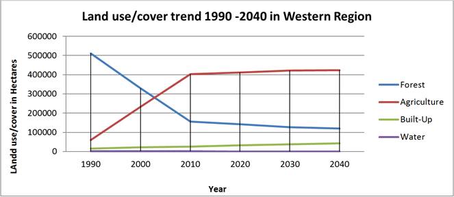
Figure 17. Land use/cover trend 1990-2040.

4. Discussion

4.1. Land Use/Cover Classification and Change Analysis

Advantageously remote sensing change detection computes the effects of anthropogenic activities on a landscape scale and does not introduce disturbances to the area under study. Especially good for ecologically sensitive areas [42]. Remote sensing ensures cost-saving and time-efficient study of landscapes essential to the management of natural resources, ecosystems, and biodiversity [2]; [7]; [41]. Remote sensing offers some of the most precise means of assessing the magnitude and pattern of changes in forest cover over a period of time [20]; [2].

Stratified random sampling was used in the selection of the training sites for the supervised classification. Stratified random sampling is by expert knowledge, the field area is strewn into strata that maximize the differences between units, and minimize the difference within each unit. One or more strata selected are estimated to be main drivers of the system under observation. A random sample is then drawn from each stratum or unit. When recognized differences exist between the strata, stratified random sampling with balanced allocation can provide improved estimation without introducing bias [36]. The biggest advantage of using stratified random sampling is that, it produces results that are both largely unbiased and accurate. Stratified often produces data that is more representative of the entire population because of the special attention it pays to the smaller subgroups within the population. It is also the best way to obtain results that reflect the diversity of the population in question. This advantage makes stratified sampling much more effective than simple sampling for large and diverse populations as the terrain in portrayed.

The overall accuracy for land use cover maps 2010, 2000 and 1990 were 79%, 78% and 80.0% correspondingly. This was deemed satisfactory for a landscape that had many variety of agricultural land, from tree crops such as cocoa, cashew, citrus, Palm; shrubs and herbaceous plants. Stratified random samplings engaged in selection of the training areas for supervised classification guaranteed that, all the variety substrata were all fittingly represented and classified duly. The overall kappa statistics for 2010, 2000 and 1990 land cover maps for ranged between 0.6 and 0.7 respectively. The results in the described analysis are of strong to moderate agreement what allows for performing further analysis and formulating valid conclusions.

The land use/cover map for 1990, 2000 and 2010 paint a very gloomy picture of forest land use category. Over 60% of forest cover is lost between 1990 -2010. Forest loss via deforestation is seen mostly outside of the protected areas. Virtually all forests outside protected area have been wiped off; they have been changed into agricultural land for cocoa cultivation mostly. Degradation of the forests is evident in the protected areas as logging, farming encroachment and illegal mining is pervasive.

4.2. Land Cover Change Analysis

Change Detection have several inferences contingent on the scope and interest of the research [34]; however, the most common understanding of the Change Detection use is its ability to provide data on changes with respects to extent, trend, location and how the change has spatially been distributed.

From 1990 to 2000, 38% and 31% for 2000-2010 correspondingly had gone through intense changes which were caused by anthropogenic forces. Agriculture is seen as the dominant land use type at 70% in 2010 surging from a measly 10% in 1990. Inferences from the figures posit that, changes that had transpired were mostly the conversion of forests into agricultural land use signifying the influences of human activities on the land cover.

Deforestation is observed outside the protected area, which degradation is witnessed in the many protected areas.

4.3. Projection for the Years 2020, 2030 and 2040

Markov-Cellular Automaton model preferred in this study was found to be satisfactory. The Kappa value of 79% was achieved in accuracy assessment. [24] advance that, this result is indicative of an excellent model.

The projected 2010 map though statistically deemed to be very good, when compared to the actual 2010 LULC map of the same area. Nevertheless, there were some observed differences in the spatial distribution of the disturbances in the protected reserves. Agriculture LU had been filtered off and distributed to the non-protected areas. These observed discrepancies could be ascribed to the contiguity filter applied in the modeling process. The utilization of adequate suitable maps signifying the driving factors data on the degree of impact on the land cover types in upcoming modeling reduces the risk of discrepancies [44]. Population data, meteorological data and policy data were considered in the modeling, but used the inherent factors in the 2000 and 2010 LU images.

The forecast for forest for the years 2020, 2030 and 2040 is not encouraging. All the land use classes except forests and water would be increasing. Agriculture increases from 2020- 2040 is marginal because all the possible Agricultural lands have been used up by 2010. Future expansion is Agriculture could be possible in the protected areas. This result indicates a slow rate in Built-Up LU when contrasted with earlier study by [16] similar study in the Ashanti Region of Ghana where Built-up class surge was more profound. This could be due to the fact that, the study area has no major industry; it is not a regional capital and most importantly rural. Ghana’s population tend to aggregate at urban areas [3]; [13]; [28].

5. Conclusion

The integration of Remote Sensing, GIS and Stochastic Modeling techniques to analyze and quantify the land cover changes (amount, trend and location) that have occurred within the period of 1990 and 2010 in the Western Region was deemed successful. The results indicate that, the study area had undergone extensive land cover changes. But for the protected forest reserves, no forest would be found in the year 2020 and beyond.

The making of land use/cover map was derived using standardized digital remote sensing classification techniques. A hierarchical level I land use and land cover classification which included of Forest, Agriculture, Water and Built-ups was used. The final classification accuracy was satisfactory or ‘good’ by means of standardized accuracy assessment measures.

Mapping via remote sensing method like all other methods have some limitations. Maps created by digital handling of multispectral data are never 100% accurate once they are made by computers [33]. The process of categorizing the Earth’s expansive range features into precise and often streamlined classes leads to errors by delineating boundaries around physically located features that are similar or acceptably diverse. Nevertheless, these margins can often be rectified by comprehensive statistical analysis to give suitably accurate land use and land cover maps as produced from satellite data [18]; [27]; [41].

The use of Landsat multi-temporal images and DMC to study land use/cover types was effective and economical to detect land use/cover changes at such a large-scale level.

Markov Chain analysis and Cellular Automaton used to forecast probable land use/cover map of the years 2020, 2030 and 2040 was deem satisfactory. The predictions shown a continuous increased of Agriculture ang built-ups, at the expense of forests. Though the use of Markov Chain analysis and Cellular Automaton was effective, it is noteworthy to restate the following limitations of the model:

(i)      It is computationally exhaustive.

(ii)    Forecasts were exclusively based on past history of classified LULC

(iii)   The forecasts show some hitches in the land use/cover spatially distribution.

5.1. Limitations

Two limitations were recognized in this study

i.      Challenges with satellite data availability for the exact years impacted the study. More cloud free satellite images for the areas of study would have been much better.

ii.     The modeling process was performed based on a model which have inbuilt limitation affected it predictions.

5.2. Recommendations

The following recommendations are necessary for the future.

i.      Supplementary studies must be undertaken to compare the validation of predicting land cover map where the time period between the future date and later date much shorter.

ii.     This study was based on first order Markov process for predicting the future land use/cover changes and considering the limitations mentioned in section 5.1, additional study should explore other progressive modeling methods for projecting land cover changes.

iii.   The twenty-year time span, 1990 - 2010, deliberated in this study is comparatively a short increase of time in a long history of land use dynamics, notwithstanding the changes were intense.

References

1. Abay, T. (2014). Factors Affecting Forest User’s Participation in Participatory Forest Management; Evidence from Alamata Community Forest, Tigray; Ethiopia.
2. Avelar, S., & Tokarczyk, P. (2014). Analysis of land use and land cover change in a coastal area of Rio de Janeiro using high-resolution remotely sensed data. Journal of Applied Remote Sensing, 8 (1), 083631. doi: 10.1117/1.JRS.8.083631.
3. Cobbinah, P. B., Erdiaw-Kwasie, M. O., & Amoateng, P. (2015). Africa’s urbanisation: Implications for sustainable development. Cities, 47, 62–72. doi: 10.1016/j.cities.2015.03.013.
4. Congalton, R. G. (1991). A review of assessing the accuracy of classifications of remotely sensed data. Remote Sensing of Environment, 37 (1), 35–46. doi: 10.1016/0034-4257(91)90048-B.
5. Desta, S. B. (2014). Deforestation and a Strategy for Rehabilitation in Beles Sub Basin, Ethiopia. Journal of Economics and Sustainable Development.
6. Eastman J. R. (2006) Eastman: Guide to GIS and Image Process. Clark Labs, Clark University.
7. Farwig, N., Lung, T., Schaab, G., & Böhning-Gaese, K. (2014). Linking Land-Use Scenarios, Remote Sensing and Monitoring to Project Impact of Management Decisions. Biotropica, 46 (3), 357–366. doi: 10.1111/btp.12105.
8. Feddema, J. J.; Oleson, K. W.; Bonan, G. B.; Mearns, L. O.; Buja, L. E.; Meehl, G. A.; Washington, W. M. (2005). Atmospheric science: The importance of land-cover change in simulating future climates. Science, 310, 1674–1678.
9. Foley, J. A.; Defries, R.; Asner, G. P.; Barford, C.; Bonan, G.; Carpenter, S. R.; Chapin, F. S.; Coe, M. T.; Daily, G. C. & Gibbs, H. K.; (2005). Global consequences of land use. Science, 309, 570–574.
10. Foody, G. M. (2002). Status of land cover classification accuracy assessment. Remote Sensing of Environment, 80 (1), 185–201. doi: 10.1016/S0034-4257(01)00295-4.
11. Giri, C., Zhu, Z., & Reed, B. (2005). Comparative analyses of the Global land Cover 2000 and MODIS land cover data sets, Remote Sensing of Environment, 94, pp 123-132.
12. Guan D; Li H; Inohaec T; Su W; Nagaiec T; Hokao K. (2011). Modeling urban land use change by the integration of cellular automaton and Markov model, Ecological Modelling 222 (2011) 3761– 3772, doi: 10.1016/j.ecolmodel.2011.09.009.
13. Hathi, P., Haque, S., Pant, L., Coffey, D., & Spears, D. (2014). Place and Child Health: The Interaction of Population Density and Sanitation in Developing Countries.
14. Kalema, V. N., Witkowski, E. T. F., Erasmus, B. F. N., & Mwavu, E. N. (2014). The Impacts Of Changes In Land Use On Woodlands In An Equatorial African Savanna. Land Degradation & Development, n/a–n/a. doi: 10.1002/ldr.2279.
15. Kissinger, G., & Herold, V. D. S. (2014). Drivers of Deforestation and Forest Degradation: A Synthesis Report for REDD+ Policymakers.
16. Koranteng, A., & Zawila-Niedzwiecki, T. (2015). Modelling forest loss and other land use change dynamics in Ashanti Region of Ghana. Folia Forestalia Polonica, 57 (2), 96–111. doi: 10.1515/ffp-2015-0010.
17. Lambin, E. F., Geist, H. J., & Lepers, E. (2003). Dynamics Of Land -Use And Land -Cover Change In Tropical Regions. Annual Review of Environment and Resources, 28 (1), 205–241. doi: 10.1146/annurev.energy.28.050302.105459.
18. Lillesand, T., Kiefer, R. W., & Chipman, J. (2014). Remote Sensing and Image Interpretation. John Wiley & Sons..
19. Medrilzam, M., Dargusch, P., Herbohn, J., & Smith, C. (2013). The socio-ecological drivers of forest degradation in part of the tropical peatlands of Central Kalimantan, Indonesia. Forestry, 87 (2), 335–345. doi: 10.1093/forestry/cpt033.
20. Miller, J. H. (1998). Active nonlinear tests (ANTs) of complex simulation models. Management Science 44 (6): 820-830.
21. Michetti, M., & Zampieri, M. (2014). Climate–Human–Land Interactions: A Review of Major Modelling Approaches. Land, 3 (3), 793–833. doi: 10.3390/land3030793.
22. Mishra, V. N., Rai, P. K., & Mohan, K. (2014). Prediction of land use changes based on land change modeler (LCM) using remote sensing: A case study of Muzaffarpur (Bihar), India. Journal of the Geographical Institute Jovan Cvijic, SASA, 64 (1), 111–127.
23. Moghadam H S; Helbich M. (2013). Spatiotemporal urbanization processes in the megacity of Mumbai, India: A Markov chains-cellular automata urban growth model, Applied Geography 40 (2013) 140e149,
24. Monserud, R. A. and Leamans, R., (1992) Comparing global vegetation maps with the kappa statistic. Ecological Modelling. Vol. 62, pp. 275-293.
25. Monson, R. K. (Ed.). (2013). Ecology and the Environment. New York, NY: Springer New York. doi: 10.1007/978-1-4614-7612-2.
26. Mousivand, A. J., Alimohammadi Sarab, A., Shayan, S., (2007). A new approach of predicting land use and land cover changes by satellite imagery and Markov chain model (Case study: Tehran). MSc Thesis. Tarbiat Modares University, Tehran, Iran.
27. Nigatu Wondrade, Dick, Ø. B., & Tveite, H. (2014). GIS based mapping of land cover changes utilizing multi-temporal remotely sensed image data in Lake Hawassa Watershed, Ethiopia. Environmental Monitoring and Assessment, 186 (3), 1765–80. doi: 10.1007/s10661-013-3491-x.
28. Obeng-Odoom, F. (2014). Sustainable Urban Development in Africa? The Case of Urban Transport in Sekondi-Takoradi, Ghana. American Behavioral Scientist, 59 (3), 424–437. doi: 10.1177/0002764214550305.
29. Overmars, K. P., & Verburg, P. H. (2006). Multilevel modelling of land use from field to village level in the Philippines. Agricultural Systems, 89 (2-3), 435–456. doi: 10.1016/j.agsy.2005.10.006.
30. Potter, C., Genovese, V., Gross, P., Boriah, S., Steinbach, M., & Kumar, V. (2007). Revealing land cover change in California with satellite data. EOS, Transactions, American Geophysical Union, 88 (26), 269.
31. Razavi, B. S. (2014). Predicting the Trend of Land Use Changes Using Artificial Neural Network and Markov Chain Model (Case Study: Kermanshah City), 6 (4), 215–226.
32. Riebsame, W. E., Meyer, W. B., and Turner, B. L. (1994). Modeling Land-use and Cover as Part of Global Environmental Change. Climate Change. Vol. 28. p. 45.
33. Robinove, C. J., (1986). Spatial diversity index mapping of classes in grid cell maps, Photogrammetric Engineering 6. Remote Sensing, 52: 1171-1173.
34. Singh, A. (1989). Digital Change Detection Techniques Using Remotely Sensed Data. International Journal of Remote Sensing. Vol. 10, No. 6, pp. 989-1003.
35. Smits P. C., Dellepiane S. G., Schowengerdt R. A. (1999). Quality assessment of image classification algorithms for land-cover mapping: a review and a proposal for a cost-based approach. International Journal of Remote Sensing, 20, 1461-1486.
36. Snedecor, G, W. & Cochran, W. G. (1989), Statistical Methods, Eighth Edition, Iowa State University Press.
37. Srivastava, P. K., Han, D., Rico-Ramirez, M. A., Bray, M., & Islam, T. (2012). Selection of classification techniques for land use/land cover change investigation. Advances in Space Research, 50 (9), 1250–1265. doi: 10.1016/j.asr.2012.06.032.
38. Tang. J., Wang, L., & Yao, Z. (2007). Spatio‐temporal urban landscape change analysis using the Markov chain model and a modified genetic algorithm, International Journal of Remote Sensing, 28: 15, 3255-3271, DOI: 10.1080/01431160600962749.
39. Voogt J. A. and Oke T. R. (2003). Thermal remote sensing of urban climates. Remote Sensing and Environment 86, 370-384.
40. Wang, Q., Shi, W., & Atkinson, P. M. (2014). Sub-pixel mapping of remote sensing images based on radial basis function interpolation. ISPRS Journal of Photogrammetry and Remote Sensing, 92, 1–15. doi: 10.1016/j.isprsjprs.2014.02.012.
41. Wang, Y., Wang, S., Yang, S., Zhang, L., Zeng, H., & Zheng, D. (2014). Using a Remote Sensing Driven Model to Analyze Effect of Land Use on Soil Moisture in the Weihe River Basin, China. IEEE Journal of Selected Topics in Applied Earth Observations and Remote Sensing, 7 (9), 3892–3902. doi: 10.1109/JSTARS.2014.2345743.
42. Willis, K. S. (2015). Remote sensing change detection for ecological monitoring in United States protected areas. Biological Conservation, 182, 233–242. doi: 10.1016/j.biocon.2014.12.006.
43. www.ghana.gov.gh
44. Zamyatin A., Markov N. (2005). Approach to land cov- er change modelling using the cellular automata // Proceedings of 8 Conference on Geographic Information Science, Estoril, Portugal, AGILE, 587–592.
45. Zhang, X., Yan, G., Li, Q., Li Z-L., Wan H., Guo Z. (2006). Evaluating the fraction of vegetation cover based on NDVI spatial scale correction model. International Journal of Remote Sensing, 27, 5359-5372.