
American Journal of Information Science and Computer Engineering, Vol. 2, No. 5, September 2016 Publish Date: Jul. 27, 2016 Pages: 45-52
A Proposal on the 3D Visualization and 3D Mapping of Knowledge Structure
Simon S. Li1, 2, Xia Lin3, Fred Y. Ye1, 2, *
1School of Information Management, Nanjing University, Nanjing, China
2Jiangsu Key Laboratory of Data Engineering and Knowledge Service, Nanjing, China
3College of Computing and Informatics, Drexel University, Philadelphia, USA
Abstract
Compared with 2D technology, the 3D visualization and 3D mapping could provide a new technical methodology for information visualization, knowledge visualization and science mapping. In this article, the 3D visualization and 3D mapping are realized by using software tools Mage and Mayavi while drawing 3D graph. The 3D graph can rotate and move in the space for visualizing knowledge structure, with keeping 3D drawing three theorems. Two cases are shown in the article: one case is the two layers network; the other belongs to three layers network. With the revealing of the 3D core structures of multilayer networks, the information and knowledge visualization and science mapping have the potential to be promoted.
Keywords
3D Visualization, 3D Mapping, Information Visualization, Knowledge Visualization, Science Mapping, H-crystal,
Knowledge Structure
Received: June 26, 2016
Accepted: July 11, 2016
Published online: July 27, 2016
@ 2016 The Authors. Published by American Institute of Science. This Open Access article is under the CC BY license. http://creativecommons.org/licenses/by/4.0/
Contents
1 Introduction
Early in the 1970s and 1980s, the visualization method began to sprout [1-2]. Since 1990s, visualization method had its scientific foundation [3-6]. After 2000, the visualization technology developed quickly and then became a new field as information visualization or science mapping [7-9]. The visualization can be used in tracking the latest developments in science and technology [10], marking the growth of scientific knowledge [11], and supporting users in coping with complexity in knowledge- and information-rich scenarios [12].
In the visualization, data visualization, information visualization, and knowledge visualization indicate different levels of abstraction [10]. The networks and knowledge maps can be depicted differently by choosing different information as the network actor, e.g. author, institute or country keyword, to reflect knowledge structures in micro-, meso-, and macro-levels, respectively [13]. Knowledge visualizing could visualize the entire body of scientific knowledge, as well as a knowledge domain’s intellectual structures that extracts structural patterns from the scientific literature and represents them in a 3-dimensional (3D) knowledge landscape [14]. Knowledge visualizing could also visualize the evolving interdisciplinary areas of science, charting, mining, analyzing, sorting, thus enable navigating and displaying knowledge [15], as well as the evolution over time about research topic [16]. Also, the types of knowledge visualization included conceptual diagrams or visual metaphors [17], concept map-based knowledge models [18], knowledge network [19], and visual concept explorer [20].
In the studies of information visualization, knowledge visualization and science mapping, technology-driven achievements have got great progress, especially when 2-dimensional (2D) software has been applied, such as CiteSpace [7], VOS viewer [21], and so on [22]. Meanwhile, the visualizing tools of multilayer networks have been developed, such as MuxViz [23], MultiNets [24] and Detangler [25].
However, most information visualization tools focus on the 2D structure. In this paper, following the study of Li et al. [26], it is suggested to pay attention to 3D visualization and 3D mapping, for promoting information and knowledge visualization and science mapping.
2. Methodology
Science mapping provides a novel perspective to reveal the scientific frontiers and dynamic structure with visualization methods [3-4,7,8,27,30]. The visualization is also a possible application of graph drawings [31].
2.1. Basic Methods and Three Theorems for 3D Drawings
It is important to draw nodes (vertices) and edges in 3D space for 3D visualization and 3D mapping, It is also named as the 3D drawings. In the 3D drawings, straight-line crossing-free drawings, whose vertices are located at points in space, are called 3D (straight-line) grid drawings. The relaxation, where edges are represented with polygonal chains with bends (if any), also at grid-points gives rise to the so-called 3D polyline grid drawings. Here, a point where a polygonal chain changes its direction is called a bend. Straight-line grid drawings are thus a special case of polyline grid drawings. Polyline drawings provide great flexibility. In particular, they allow 3D drawings with smaller volume than that in the straight-line model. The number of bends, however, should be kept as small as possible, since bends typically reduce the readability of a drawing. If each segment of each edge in a polyline drawing is parallel to one of the three coordinate axes, then the drawing is an orthogonal drawing. Orthogonal drawings are thus special cases of polyline drawings.
Since 3D grid drawings have straight edges and no crossings, the volume is the main aesthetic criterion for this drawing style. In other words, the most commonly used measure for 3D grid drawings is their volume. There are three theorems for clarifying the key.
A starting point for many results on 3D grid drawings is a simple fact, i.e., a straight-line drawing of a graph (on n > 3 vertices) such that no four vertices are coplanar without crossings. This fact is the key to the folklore construction that proves that every graph has a 3D grid drawing. In particular, a moment curve M is a curve defined by parameters (q, q2, q3).
It can be proved that no four distinct points on this curve are coplanar. Thus given a graph G on n vertices, a 3D grid drawing of G can be obtained by placing each vertex vi ![]() (G), 1 ≤ i ≤ n, at (i, i2, i3). This construction gives an n × n2 × n3 3D grid drawing with O (n6) volume. By placing each vertex vi at the grid-point (i, i2 mod p, i3 mod p), where p is a prime such that n < p ≤ 2n, the resulting drawing is an n × 2n × 2n 3D grid drawing with O (n3) volume. Furthermore, Cohen et al. (1996) proved that the Ω(n) × Ω(n) × Ω(n) bounding box and thus the Θ(n3) volume bound is asymptotically optimal in the case of the complete graph Kn. The proof of this lower bound is based on the fact that no five vertices can be coplanar in any 3D grid drawing of Kn. Therefore, each side of the bounding box has size at least n/4, as the following Cohen-Eades-Lin-Ruskey Theorem illustrates [32].
(G), 1 ≤ i ≤ n, at (i, i2, i3). This construction gives an n × n2 × n3 3D grid drawing with O (n6) volume. By placing each vertex vi at the grid-point (i, i2 mod p, i3 mod p), where p is a prime such that n < p ≤ 2n, the resulting drawing is an n × 2n × 2n 3D grid drawing with O (n3) volume. Furthermore, Cohen et al. (1996) proved that the Ω(n) × Ω(n) × Ω(n) bounding box and thus the Θ(n3) volume bound is asymptotically optimal in the case of the complete graph Kn. The proof of this lower bound is based on the fact that no five vertices can be coplanar in any 3D grid drawing of Kn. Therefore, each side of the bounding box has size at least n/4, as the following Cohen-Eades-Lin-Ruskey Theorem illustrates [32].
Cohen-Eades-Lin-Ruskey Theorem: Every n-vertex graph has a 3D grid drawing with O(n3) volume. Moreover, the bounding box of every 3D grid drawing of Kn, the complete graph on n vertices, is at least (n/4) × (n/4) × (n/4), and thus has (n3) volume.
This construction provides a generalization of an analogous 2D technique.
Since complete graphs require cubic volume, it is of interest to identify fixed graph parameters that enable 3D grid drawings with smaller volume. The first parameter to be studied is the chromatic number [33-34]. Calamoneri and Sterbini [33] proved that each 4-colorable graph has a 3D grid drawing with O(n2) volume. Generalizing this result, Pach et al. [34] proved the following Pach-Thiele-Toth Theorem.
Pach-Thiele-Toth Theorem: Every n-vertex graph with chromatic number χ has a 3D grid drawing with O(χ2n2) volume. This bound is asymptotically optimal for the complete bi-partite graphs with equal sized bipartitions.
The main idea behind this result is similar to that for general graphs. In the case of complete graphs, crossings are avoided by ensuring that no four vertices are coplanar.
Following the Pach-Thiele-Toth Theorem, which proved that the quadratic volume bound is asymptotically optimal for the complete bipartite graph with equal sized bipartitions, Bose et al. gave a generalized result for all graphs as another theorem [35].
Bose-Czyzowicz-Morin-Wood Theorem: Every 3D grid drawing with n vertices and m edges has volume at least (n + m)/8. In particular, the maximum number of edges in an X × Y × Z drawing is exactly (2X − 1)(2Y − 1)(2Z − 1) − XYZ.
The above theorems are the principle theorems for 3D drawing, which should be taken into consideration in 3D visualization. Meanwhile, in 3D molecular technologies, some synthetic software tools have been developed, such as VEGA [36] and POSMOL [37], which provide rich and variable references. However, in molecule networks, all nodes are atoms and the 3D graph expresses their molecular structure. On the contrary, in 3D information networks, all nodes focus on publications or related subjects and the 3D graph reveals their knowledge structure.
2.2. Software Tools and Realizing Techniques for 3D Visualization and 3D Mapping
In order to simplify its technical process, the common shared or open source software tools are chosen for 3D Visualization and 3D Mapping. Combining above theoretical concepts with practical applications, an applicable tool package Mayavi (3D scientific data visualization and plotting in Python, cf. http://docs.enthought.com/mayavi/mayavi/) was adopted to realize the 3D visualization and 3D mapping, and Mage (3D vector display program which can show "kinemage" graphics, cf. http://kinemage.biochem.duke.edu/software/mage.php) was applied to show a real 3D graph.
It is impossible and unnecessary to draw all nodes and edges in one 3D graph. Thus, it is better to draw the core structure as 3D graph. Considering a multilayer complex network, h-crystal algorithm had been designed [26], where h-crystal in multilayer weighted information network is constructed by combining co-citation network (layer 1), bibliographic coupling network (layer 2) and co-keyword network (layer 3) as a multilayer network, which provides an operational 3D graph. In the 3D visualization and 3D mapping, the nodes in layer 1 are set as blue ball, layer 2 green cube and layer 3 red cone.
For positioning the nodes in 3D graph, we also use the "neato" distribution algorithm in Graphviz (Graph Visualization Software, cf. http://www.graphviz.org/) to fix coordinates (x, y) and give an artificial coordinate z (ex. the z of nodes in layer 1 as z1, layer 2 as z2 and Layer 3 as z3).
The generated 3D graph can be penetrated in different direction, with rotation, as shown in Figure 1.
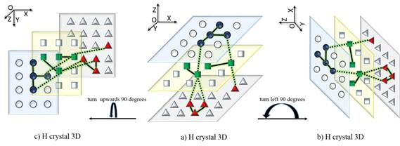
Fig. 1. The 3D graph and its core, 3 projections with rotations.
In the Figure 1, if the first projection a) is face, the second projection b) is a left-right turn 90o rotation of a) and the third projection c) is an up-down turn 90o rotation of b). Combing a), b) and c) three projections, a 3D structure of the multilayer network core can be presented. During the process, three theorems of the 3D drawing are kept.
For characterizing the core structure of 3D graph, the layer structural parameters and total structure parameter (S) for measuring total nodes and edges are introduced, as follows.
Layer structural parameters are calculated by the sum of layer core nodes and edges. For example, if the multilayer weighted network consists of two layers A, B, the sum are defined as
![]() (1)
(1)
![]() (2)
(2)
In this example, NA, NB are nodes’ symbols of layer A, B each with h-degree NAh, NBh, and the number of nodes, that node’s h-degree equals NAh, NBh, are NAd, NBd respectively. LA, LB are edges’ symbols of layer A, B each with h-strength LAh, LBh, and the number of edges that edge’s h-strength equals LAh, LBh are LAd, LBd respectively. If there are three layers, they can be respectively set as A, B and C.
Then the total structural parameter S can be defined as the sum of all core nodes and edges in all layers excluding duplicate nodes (which equals all nodes and edges of the h-crystal). For two layers, it is
![]() (3)
(3)
For three layers, it is
![]() (4)
(4)
where NAB is the number of same nodes of NAh and NBh, and NBC is that of NBh and NCh.
The larger the layer is and total structural parameters are, the more complicated the network core is.
2.3. Datasets
The empirical data are searched from WoS, including two sets: (1) dataset "sm-set", which is searched by search strategy TS=("science map*" or "knowledge map*"); (2) dataset "cn-set", which is searched by search strategy TI="complex network*". These two datasets are searched in the database WoS (1998-2013) without restriction. Data are updated on Nov.19 and Nov.7, 2014, respectively.
3. Results
Using h-crystal algorithm [26], a 3D core of knowledge structure is presented, in which there are two layers for dataset "sm-set" and three layers for dataset "cn-set".
These two data sets produce two multilayer information networks with combination of co-citation network, bibliographic coupling network and co-keyword (including the keywords in both ID and DS records) network., Their main parameters are shown in the Tables 1 and 2.
Table 1. The structural parameters of dataset "sm-set".
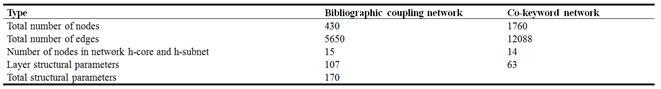
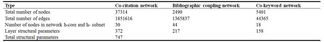
Table 2. The structural parameters of dataset "cn-set".
In order to compare different results, it is noticed that dataset "sm-set" shows a two layer 3D graph and dataset "cn-set" does a three layer 3D graph.
3.1. The 3D Graph of "sm-set"
Using the h-crystal algorithm and tool package Mayavi, "sm-set" produced a two-layer h-crystal, as shown in Figure 2, in which B means bibliographic coupling layer and C co-keyword layer. In B layer, paper node is also link-marked by author and publishing year; and in C layer, keyword is marked.

Fig. 2. The two-layer 3D graph of dataset "sm-set".
In order to present real 3D effect, the Figure 2 can also be present in another way with using Mage, as shown in the Figure 3.
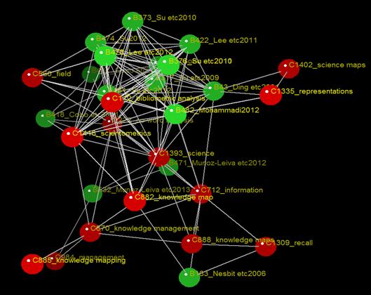
Fig. 3. The real 3D effect of "sm-set" 3D graph.
Combining Table 1 and Figure 2, it is shown that 15 core bibliographic coupling papers support 14 core keywords. Figure 3 shows the visual image, where the keywords such as ‘knowledge maps’, ‘science maps’, ‘bibliometric analysis’ are supported by those important documents.
3.2. The 3D Graph of "cn-set"
Using the h-crystal algorithm and tool package Mayavi, "cn-set" produced a three layer h-crystal, as shown in Figure 3, in which A marks co-citation layer, B means bibliographic coupling layer and C does co-keyword layer. In both A and B layers, paper node is link-marked by author and publishing year; and in C layer, keyword is marked.
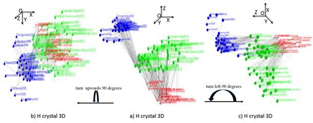
Fig. 4. The three layer 3D graph of dataset "cn-set".
For seeing real 3D effect, with using Mage, Figure 4 can be transformed into the Figure 5, as shown below.
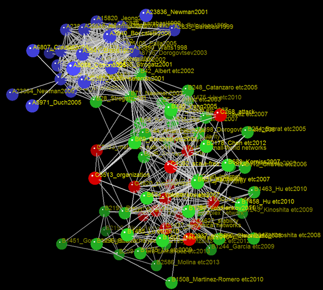
Fig. 5. The real 3D effect of dataset "cn-set".
Combining Table 2 and Figure 4, it is shown that 30 core co-citation papers link with 44 core bibliographic coupling papers, and the 44 papers support 18 core keywords. Figure 5 shows the visual image, where keywords ‘scale-free networks’, ‘metabolic networks’, ‘community structure’ etc. are supported by those important documents.
Compared with 2D visualization and 2D mapping, the 3D visualization and 3D mapping can show more detailed information. Therefore, more "cubic" structure and its construction are known.
4. Discussion
The above 3D graphs presented in this article provide real 3D visualization, in which we can turn and rotate the graphs for viewing of different directions. With its advantages, the 3D visualization technology could provide following applications.
(1)The 3D graphs can reveal the space structure of network core, which might supply a new research way to investigate the inner structure of information networks and other networks.
(2) The 3D graphs can be applied to show real knowledge structure hidden in information networks, where knowledge generation and development might be revealed in dynamic cases.
(3) The 3D graphs may push forward the development of visualization technologies, particularly in the studies of multilayer and multiplex networks [23].
Certainly, it also has limitations. The method of the 3D graph is restricted to process smaller dataset, so that we can only use it to show ‘core information’ or ‘core knowledge’. For processing ‘bigdata’, more efforts are needed in order to find other ways.
5. Conclusion
3D visualization and 3D mapping of knowledge structure can be realized by 3D graph technology developed in the article, on which the examples of core structure of multilayer information networks at both two-layer case and three-layer case are shown. Meanwhile, the three theorems of 3D drawing are kept.
As the 3D graphs can show detailed structural information, the real knowledge structure and its construction can be visual presentations as space images. It is expected that the visualization technology is useful in 3D graphics, particularly for 3D visualization and 3D mapping such as molecular structure and complex network. The 3D visualization and 3D mapping could stimulate and promote the development of information visualization, knowledge visualization and science mapping.
Acknowledgements
We acknowledge the National Natural Science Foundation of China Grant No 71173187 and Jiangsu Key Laboratory Fund for financial supports, and thank Dr. Xuguang Li for English proofreading.
References
- H. Small, B. C. Griffith, The structure of scientific literatures I: Identifying and graphing specialties, Science Studies, 4(1), 17–40(1974).
- H. Small, E. Garfield, The geography of science: Disciplinary and national mappings, Journal of Information Science, 11(4), 147–159(1985).
- K. McCain, Mapping economics through the journal literature: An experiment in journal co-citation analysis, Journal of the American Society for Information Science, 42(4), 290–296(1991).
- E. Garfield, Scientography: Mapping the tracks of science, Current Contents: Social & Behavioural Sciences, 7(45), 5–10(1994).
- H.D. White, K. W. McCain, Visualizing a Discipline: An Author Co-Citation Analysis of Information Science, 1972–1995, Journal of the American Society for Information Science, 49(4), 327–355 (1998).
- H. Small, Visualizing science by citation mapping, Journal of the American Society for Information Science, 50(9), 799–813(1999).
- C. Chen, CiteSpace II: Detecting and Visualizing Emerging Trends and Transient Patterns in Scientific Literature, Journal of the American Society for Information Science and Technology, 57(3), 359–377 (2006).
- E. Garfield, A.I. Pudovkin and V.S. Istomin, Why Do We Need Algorithmic Historiography? Journal of the American Society for Information Science and Technology, 54(5), 400–412(2003).
- H. Small, Paradigms, Citations, and Maps of Science: A Personal History, Journal of the American Society for Information Science and Technology, 54(5), 394–399 (2003).
- M. Chen, D. Ebert, H. Hagen, et al, Data, information, and knowledge in visualization,IEEE Computer Graphics and Applications, 29(1), 12-19(2009).
- C. Chen, Visualization of knowledge structures, Handbook of software engineering and knowledge engineering, 2002, 2, 201-238(2002).
- T. Keller, S. O. Tergan, Visualizing knowledge and information: An introduction, Knowledge and information visualization, Springer Berlin Heidelberg, 1-23(2005).
- H. N. Su, P. C. Lee, Mapping knowledge structure by keyword co-occurrence: a first look at journal papers in Technology Foresight, Scientometrics, 85(1), 65-79(2010).
- R. J. Paul, Visualizing a knowledge domain’s intellectual structure, IEEE Computer, 34(3), 65-71(2001).
- R. M. Shiffrin, K. Börner, Mapping knowledge domains, Proceedings of the National Academy of Sciences, 101, 5183-5185(2004).
- J. Zhang, J. Xie, W. Hou, et al, Mapping the knowledge structure of research on patient adherence: knowledge domain visualization based co-word analysis and social network analysis, PloS one, 7(4), e34497(2012).
- M. Eppler, R. Burkhard, Knowledge visualization, Encyclopedia of knowledge management, 551-560(2005).
- A. J. Cañas, R. Carff, G. Hill, et al. Concept maps: Integrating knowledge and information visualization, Knowledge and information visualization. Springer Berlin Heidelberg, 205-219(2005).
- J. Sun, P. Zhang, Visualization of researcher's knowledge structure based on knowledge network, Industrial Engineering and Engineering Management, 2067-2071(2009).
- X. Lin, D. Zhang, Visualization of Knowledge Structures, 11th International Conference Information Visualization, 476-484(2007).
- N.J. van Eck, L. Waltman, Software survey: VOSviewer, a computer programfor bibliometric mapping, Scientometrics, 84, 523–538(2010).
- M.J. Cobo, A.G. López-Herrera, E. Herrera-Viedma and F. Herrera, Science Mapping Software Tools: Review, Analysis, and Cooperative Study Among Tools, Journal of the American Society for Information Science and Technology, 62(7), 1382–1402(2011).
- M. De Domenico, M. A. Porter, A. Arenas, MuxViz: a tool for multilayer analysis and visualization of networks, Journal of Complex Networks, 3 (2): 159-176 (2014).
- M. Piškorec, B. Sluban, T. Šmuc, MultiNets: Web-Based Multilayer Network Visualization, In Machine Learning and Knowledge Discovery in Databases, Springer International Publishing (2015).
- B. Renoust, G. Melancon, T. Munzner, Detangler: Visual Analytics for Multiplex Networks, In Computer Graphics Forum, 34(3), 321-330 (2015).
- S.S. Li, X. Lin, X. Liu and F. Y. Ye, H-crystal as a Core Structure in Multilayer Weighted Networks, American Journal of Information Science and Computer Engineering (2016) (in press).
- X. Lin, H. D. White, J. Buzydlowski, Real-time author co-citation mapping for online searching, International Journal of Information Processing & Management, 39(5), 689-706(2003).
- K. Börner, S. Sanyal, A. Vespignani, Network science, Annual Review of Information Science and Technology, 41, 537-607 (2007).
- L. Leydesdorff, O. Persson, Mapping the geography of science: Distribution patterns and networks of relations among cities and institutes, Journal of the American Society for Information Science and Technology, 61(8), 1622–1634 (2010).
- X. Lin, J. Ahn, Challenges of knowledge structure visualization, Proceedings of the International UDC Seminar 2013, 73-87(2013).
- R. Tamassia, Handbook of graph drawing and visualization, CRC press(2013).
- R. F. Cohen, P. Eades, T. Lin and F. Ruskey, Three-dimensional graph drawing, Algorithmica, 17(2),199–208(1996).
- T. Calamoneri, A. Sterbini, 3D straight-line grid drawing of 4-colorable graphs, Information Processing Letter, 63(2), 97–102 (1997).
- J. Pach, T. Thiele, G. Toth, Three-dimensional grid drawings of graphs, Contemporary Mathematics, 223, 251-256 (1999).
- P. Bose, J. Czyzowicz, P. Morin and D.R. Wood, The maximum number of edges in a three-dimensional grid-drawing, Journal of Graph Algorithms and Applications, 8(1), 21–26(2004).
- A. Pedretti, L. Villa, G. Vistoli, VEGA: a versatile program to convert, handle and visualize molecular structure on Windows-based PCs, Journal of Molecular Graphics and Modelling, 21, 47–49(2002).
- S. J. Lee, H. Y. Chung, K.S. Kim, An Easy-to-Use Three-Dimensional Molecular Visualization and Analysis Program: POSMOL, Bulletin of Korean Chemical Society, 25(7), 1061-1064(2004).


