Energy-Efficient Routing Protocols in Presence of the Mobile Sink in Wireless Sensor Networks

Bahadorani Mahjobeh^{1, *}, Jamali Shahram²

¹Faculty of Technical and Engineering, Islamic Azad University, Ardabil, Iran

²Department of Computer Engineering, University of Mohaghegh Ardabili, Ardabil, Iran

Abstract

Wireless sensor networks (WSN) consist of small-sized sensor nodes and inexpensive short-range radio communication. One of the known features in wireless sensor nodes is the limited battery supply. On the other hand, replacing the battery in wireless sensor networks is difficult and often is impossible. Therefore, it is essential to employ an energy- efficient routing protocol for minimizing energy consumption in these networks. In this paper, we provide a deeper understanding of energy- efficient routing protocol for mobile sink. We describe the reduction factors of energy in wireless sensor networks. Moreover, the sink node mobility explain, which it is one of the most challenging factors in the energy consumption of these networks. Then, discuss a comprehensive survey about various energy strategies and protocols in the sink node mobility. These energy- efficient routing protocols can be class based on their performance, into two categories such as: source- initiated and sink-initiated. For each category, we present several examples of protocols. In each samples, protocol pay the sink node mobility and energy storage. Also, with comparing the protocols to each other, we can emphasize on the advantages and disadvantages of each sample protocols.

Keywords

Energy-Efficient, Sink Mobility, Routing Protocol, Wireless Sensor Network

Received: July 12, 2015
Accepted: July 25, 2015
Published online: August 17, 2015

@ 2015 The Authors. Published by American Institute of Science. This Open Access article is under the CC BY-NC license. http://creativecommons.org/licenses/by-nc/4.0/

1. Introduction

A wireless sensor network consists of a number of sensor is equipped with limited battery power and short- range radio communication [1]. Because of limited resource, one of the important issues that can be considered in the design of the sensor network routing protocols, as much as possible to be preserved the level of energy in every phase of the network operations. In fact, energy is the main resource for sensor networks. Due to the difficult to recharge batteries in thousands of the sensor nodes are distributed in remote and difficult environments. Various factors may be caused the waste of the limited resource of energy in sensor networks that they include:

Interference: it is from the inherent characteristics of the sensor network and it causes the data collision, the data retransmission, thus a significant waste of energy is occurred because it is the unsuccessful transmissions [2].

Data Redundancy: sensor nodes may significantly produce the data redundancy. This means that multiple nodes can be created similar packets so that send the same data to reduce the energy in the wireless sensor network [3].

Accuracy level: the purpose of communication in wireless sensor network is data reporting and data processing. In the data reporting, the amount of the received data determines the accuracy of the data [4]. So in the critical applications that rely on the measurement results, the accuracy level is a key factor. On the other, receiving more data in order to increase level of accuracy, can consume more energy.

Sink node mobility: mobility nodes such as the sink node in a sensor network causes energy drain within sensor network. In this paper, we discuss about the factor of energy dissipation of the sensor network and in the presence of the mobility sink node, consider a classification of energy - efficient protocols.

Then we will review protocols in each classes in most applications of wireless sensor networks, sensor nodes are fixed. But, there are important applications in which the nodes such as sink node can are mobile. However, a few researches have examined the sink node mobility [5]. The applications of the sink node mobility are as follows:

A soldier on the battlefield and the enemy territory, while collecting data and tracking of the enemy mobile soldiers or the mobile enemy tanks. Users gathering traffic information from a large scale WSN deployed in a metropolis while driving [5]. Also, in the home networking that consumer products can collect and transmit various types of data in the home environment [6] and a group of mobile robot in a WSN to monitor the level of radioactive or chemical pollutions used in some environments.

When the sink moves, frequent location updates from the sink can generate excessive power consumption of sensors [5]. Hence, when there are multiple sink nodes in a sensor network more energy drains in a sensor network. Therefore, are needed the energy - efficient routing protocol in the presence of mobile sink nodes.

We aim to provide a deeper understanding of energy- efficient routing protocol for mobile sink and also identified some issues have worthy of more survey.

This paper is organized as follows, section 2 and 3, respectively, provide classify and comprehensive review of energy- efficient protocols for wireless sensor networks in the presence of the mobile sink node. In section 4, express comparing protocols with each other. In section 5, we expressed the results of this study.

2. Energy-Efficient Routing Protocols in the Presence of the Mobile Sink Node

In this section, routing protocols in the field of energy efficiency in wireless sensor networks with mobile sink node will be reviewed and they will be provided the classification. In this paper, the routing protocols are divided in two categories, source-initiated protocol and sink-initiated. The classification is shown in figure 1.

Fig. 1. Routing protocols categories.

2.1. Source-Initiated Protocol

In source-initiated protocol accept members and the algorithm starting is from side the source node. Although these methods have advantage in support of the sink node mobility, but there are inefficient when the source node is moving. The number of sources also affects the performance. In this paper, these methods according to their performance are presented as follows.

2.1.1. Grid Method

At the beginning of the algorithm, every fixed source node, rather than waiting to receive sink’s the new location message, it starts operations and in wireless sensor network creates the grid structure included of cells. So that, every mobile sink node requires its information message distributes only within the small confine of the cell size. For example, TTDD [3] protocol used the grid method, that in the next section we describe it.

2.1.2. Tree Method

In this method, the algorithm starts from the source node. Some protocols that use this method are effective in high density network and some those are used mobile sink node as members of the tree. Due to the sink node mobility, frequent changes are produced in the diffusion branches of tree. Also, some older protocols during tree construction, only attention to minimum geographical distance parameter. When the sink’s desired refresh rate is different, this parameter will not be the best choice to connect sink node to the tree. Unlike the old protocols a protocol as SEAD [7], for connect sink node to the tree considers both the minimum geographical distance and the sink’s desired refresh rate. Also, don’t use the mobile sink node as intermediate members of the tree. SEAD protocol will be described in the next section.

2.2. Sink-Initiated Protocol

In sink- initiated protocol accept members are from side sink node. Unlike source-initiated protocol, not rely on the source node. That are inefficient if mobility of the source node, it is not affected by number of the sources in its signal overhead. These methods are presented as follows according to their performance.

2.2.1. Data-Centric Method

In this method for publishing data between the source node and the sink node, is done accepting members from the sink node. This is the early work of the data publishing on wireless sensor network in presence of the mobile node. In this method, due to the low ability of sensor nodes and not aware of location information, all communications and creating paths in the sensor network are based on data. DD [8] protocol is including the protocols that are used this method and we will explain it.

2.2.2. Rendezvous-Based Method

This method is a sink-initiated protocol so accept member from side the sink node. Since the sink node is mobile, the problem with collecting data directly from sensor nodes is that it becomes impractical when there are a large number of sensor nodes. Visiting each sensor node increases the mobile sink’s traveling path length and results in sensor nodes experiencing buffer overflow due to data collection delays. To address this problem, researchers have proposed a rendezvous-based model, in which a mobile sink only visits a subset of sensor nodes called RPs (rendezvous points). The sensor nodes outside the mobile sink path send their data via multihop communications to these RPs. The main goal of protocols in this category is to find a subset of RPs to minimize energy consumption. Protocols such as: IAR, ERMMSDG [9], WRP [10] uses this method. We will explain these Protocols in next section.

3. Describe Different
Energy-Efficient Routing Protocols When There Is Mobile Sink

3.1. Source-Initiated Routing Protocols

In this section, we describe source- initiated protocols.

3.1.1. TTDD Protocol

It is a Two-Tier Data Dissemination protocol. It is formed of three original sections such as: grid construction, two-tier query and data forwarding, grid maintenance.

A.  Grid construction

Upon detection of a stimulus in the wireless sensor field, the source node divides the sensor field into a grid of cells. The crossing point of the grid calculates the following equation:

L_P= (X_i, Y_j)= {X_i= X+i.α, Y_j= Y+j.α; i,j=±0, ±1, ±2,…}  (1)

Where is:

α: cell size.

(X, Y): location of source.

(Xi, Yj): location of grid points.

The source sends a message to the four neighbor points on the grid using simple greedy geographical forwarding (GF). Then checks at a node that is closer to LP than other its neighbors, if this node’s distance to LP is less than a threshold α/2, it calls as dissemination node. Otherwise, the node simply drops the message. A dissemination node stores a few pieces of information for the grid structure, including the dissemination point LP it is serving and the upstream dissemination node's location.

B.  The two-tier query and data forwarding

In fact, forwarding a query performs in two tiers. The lower tier is within the local grid cell of the sink's current location, and the higher tier is made of the dissemination nodes at grid points.

Fig. 2. Two-tier query and data forwarding.

When a sink needs to data, in order to detection the immediate dissemination node it sends the local query into its cell by flooding. Then this dissemination node forwards the query message to upstream dissemination node. This process continues until it reaches either the source or a dissemination node that is already receiving data from the source. Once a source receives the query message from it’s the neighbor dissemination node, data sends to it. Then this dissemination node forwards data to the downstream node and finally to the sink’s primary dissemination node (Initially the primary and immediate dissemination node are the same sensor node). See figure 2 for an illustration. Two- tier query and data forwarding between Source A and Sink S₁, S₂. Sink S₁ starts with flooding its query with its primary agent PA's location, to its immediate dissemination node D_S. D_S records PA's location and forwards the query to its upstream dissemination node until the query reaches A. The data are returned to D_S along the way that the query traverses. D_S forwards the data to PA, and finally to Sink S₁. Similar process applies to Sink S₂, except that its query stops on the grid at dissemination node G.

When a sink is about to move out of the range of its primary dissemination node/agent, it chooses the neighboring node that has the strongest signal-to-noise ratio as its new immediate agent and sends the location of the new immediate agent into its query. The primary agent deliveries data to the immediate agent and also it sends data to sink. If sink moves out of the immediate agent’s range, it will again choose an immediate agent at the new location. For more details see figure 3.

Fig. 3. Trajectory forwarding.

C.  Grid maintenance

A source includes a grid lifetime in the message sends to the neighbor nodes (when to build the grid). If the lifetime elapses and the dissemination nodes on the grid do not receive any further data announcements to extend the lifetime, they clear their states and the grid no longer exists. Moreover assuming the failure of the sensor nodes, do not periodically refresh the grid during its lifetime. Instead, TTDD employs an upstream information duplication mechanism in which each dissemination node replicates in the neighborhood sensor nodes the location of its upstream dissemination node. When this dissemination node fails, one of them is to be replaced.

3.1.2. SEAD Protocol

SEAD focuses on dissemination in which a source sends its data to multiple sinks. It is consists of two parts: d-tree construction and d-tree management.

This protocol does not use mobile sinks as intermediate members of the tree. This precludes frequent changes of the dissemination path due to sink mobility. Also, each branch of the tree may have its update rate so that depends on the desired refresh rates of the branch’s downstream sink.

When a mobile sink wants to join the dissemination tree (d-tree), it selects closest its neighboring sensor nodes to send a join query to the source of the tree. It is called the sink’s access node.

The join query message contains the location of the access node A_i and the sink’s desired update rate R_i. The access node delivers the data to the sink without exporting the sink’s location information to the rest of the tree. The tree is updated only when the access node changes (as opposed to every time some node moves). As the sink moves, no new access node is chosen until the hop count between the access node and the sink exceeds a threshold. The value of this threshold allows trade-offs to be made between path delay and energy spent on reconstructing the tree.

A replica defines as a sensor node temporarily stores the latest data incoming from the source and asynchronously disseminates it to others along the tree. Figure 4 shows the above definitions.

Fig. 4. An example of the SEAD d- tree model in the sensor network.

A.  D- Tree construction

SEAD protocol starts when a source receives a query indicating a sink’s desired refresh rate. D- Tree construction consists of three phases: subscription query, gate replica search, replica placement.

At the subscription query phase, a sink directs a join query to the source via its access node. At the gate replica search phase, a gate replica is determined, which serves as the grafting point (on the existing tree) from which a branch to the new access point is extended. In this phase for search the gate replica in order to minimize energy is considered the following equation. In other words, both proximity and desired sink refresh rate must be considered:

Energy_cost (a, b) ∝ d(a,b) Pab                       (2)

Where P_ab is the packet sending rate and d(a,b) is distance between a and b nodes.

The replica placement phase locally readjusts the tree in the neighborhood of the gate replica to further reduce communication energy. In this phase there are two ways to connect the access node to the gate replica. One is to connect it as a child of the gate replica. This option adds no replicas to the tree, and is called "non-replica" mode. The other is to create a child for the gate replica to feed the access node and some of the gate replica’s original children. It is called "junction" mode. The replica placement phase calculates the cost of two modes and compares with together. Then selects the better mode so that the access node joins the tree in a way that minimizes the energy cost. According to equation (2) for calculating the energy cost should be considered both the geographical distance and the packet sending rate.

B.  D-Tree management

The second part of the protocol lies in maintaining connectivity between mobile sinks and their access nodes. So that the connection removing occurs for two reasons such as: sink mobility or leaving d-tree. In the sink mobility reason, replace the existing access node with a new access node when the sink moves far enough away. In the leaving d-tree reason, sinks ends a leave message to its access node and the access node requests its parent to delete it from its list of children and stop forwarding data to it.

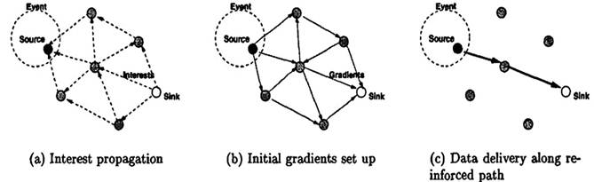
Fig. 5. The simplified schematic for DD.

3.2. Sink-Initiated Routing Protocols

In this section, we describe sink-initiated protocols.

3.2.1. DD Protocol

Sink requests data by disseminating an interest. Every node maintains an interest cache. Each entry in the interest cache has several fields, as example gradient field that it is created for each neighbor. In fact, a gradient specifies both a data rate and a direction in which to send events. When a node receives an interest, it checks to see if the interest exists in the cache. If no matching entry exists, the node creates an interest entry. If there exists an interest entry, but no gradient for the sender of the interest, the node adds a gradient with the specified value. Then node re-sends the interest to subset of its neighbors. Thus, this dissemination sets up gradients in all networks. In summary, interest propagation sets up state in the network to facilitate data towards the sink. To create gradient between sink and source, the source sends data, possibly along multiple paths, towards the sink. Among these paths, only one path is selected as the reinforcement. This selecting based on highest data rate figure 5 shows a simplified schematic for DD protocol.

Fig. 6. Setup the relay path.

3.2.2. IAR Protocol

Sink selects the closest its the neighbor node. This node is called agent (In other words, it is a RP). Then, it sends the query message only to the agent, which broadcasts it by flooding. As the query propagates, each sensor node can determine the next hop node toward the agent. Because, each query packet has a hop count field, which is updated hop-by-hop and records the distance of the transmitter of the packet. Finally, each node selects its next hop node among its neighbors that are 1 hop closer to the agent. In other words, agent based path management. So that, other nodes deliver data to agent by multiple hops and it forwards data to sink. When the sink moves out the radio range of the agent, at it’s the new location can find the closest node based on the coordinates from it’s the neighbor nodes. The closest node is called an immediate relay node (IR). The sink transmits relay path setup (RPSP) message to the agent via the selected IR. After the agent receives the RPSP, data packets are routed along the reverse path of the RPSP towards the IR. So, IR forwards the data packets to the sink. When the sink moves again out of the radio range of the IR node, it selects new IR in the same way. The IR Selecting process and the relay path setup process are shown in figure 6.

3.2.3. ERMMSDG Protocol

In this process, a biased random walk method is used to determine the next position of the sink. Then, a RP selection with splitting tree technique is used to find the optimal data transmission path. If the sink moves within the range of RP, it receives the gathered data and if moved out, it selects a relay node from its neighbours to relay packets from RP to the sink.

A.  Determination of next position and optimal path for the sink

Let CN_i, be the counter for every vertex I and ¶_i, be the degree of vertex i. Initially CN_i = 0 " i e J.

When a mobile sink S enters the area related to i, it increments the counter CN_i by 1. The subsequent position of the sink is estimated by choosing one the neighbours of the current cell. The probability of visiting neighbour vertex j is estimated using the following equation (for CN_nei≠0):

                                (3)

Where:

                             (4)

This reveals that, when the sink is located at closer region, very less frequently visited areas are preferred.

The path that needs to be traversed by the sink is determined by applying the rendezvous point selection with splitting tree technique. These steps are as follows:

1)  Initialize the tree-shaped network topology.

2)  S computes the overall in-network communication cost for each node. It is as follows:

                              (5)

Where DR(i) is the data generation rate, E(i) is the expected transmission count of the link of any node and its neighbour and h is the parameter related to energy consumption.

3)  The node with minimum TR is chosen as Median (K).

4)  The tree-shaped node topology is directed via K.

5)  Then the optimal path (P_o) is estimated using the rendezvous point with mobile sink nodes (ReP_mr).

Where A is the adjacent matrix of the tree shaped topology and B is the maximum length of mobile elements path.

6)  The P_o value is inserted into candidate set CS.

7)  The children of C is inserted into Q.

8)  The global optimal path (P_og) with minimum TR is estimated from CS.

For example, consider a tree shaped network topology as shown in Fig. 7(a). The node with minimum TR is chosen as median(K) as shown in Fig. 7(b) and Fig. 7(c) shows the optimal path P_o (2): N₁--> N₂--> N₃, P_o (3): N₅--> N₈--> N₁₀, P_o (4): N₇--> N₁₂--> N₆.

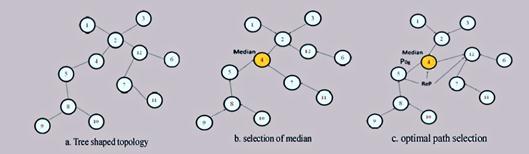
Fig. 7. Rendezvous point selection with a mobile sink.

B.  Data transmission technique

The reliable data transmission technique involves three phases: data encoding, communication and data decoding. Each static N_i, encodes the data packets by utilizing the conventional codes, such as the Reed-Solomon (RS) codes. Such that the coded data include a verbatim copy of the source elements. Thus, if there are w elements, y out of w need not be encoded which in turn reduces the memory utility. The encoding and decoding process is as follows:

1)  To maintain y value as minimum and independent from the source bundle, the source data are split into Z blocks (i.e. Z_o, Z₁, Z₂,…, Z_Z-1).

2)  Each Z block includes y data units.

3)  Each block is encoded individually to generate W data units.

4)  The ratio among number of redundant and original messages is termed as stretch factor s (s @ w/y).

5)  When a source data is ready, encoding is performed by sensor node.

6)  The sensor node now initiates the communication when it detects multiple S in its transmission distance.

7)  S after receiving the w different encoded. Message decodes the message and stores the resulting block in its local buffer.

8)  Once all Z blocks have been appropriately decoded, S obtains a copy of the original bundle.

9)  If all the necessary encoded messages are not received by the S, then the decoding is failed. Error message (EM) is transmitted to respective sensor nodes.

C.  Efficient routing protocol for data gathering

Efficient Routing Protocol for Multiple Mobile Sink Based Data Gathering (ERMMSDG) technique is as follows:

1)  The tree-shaped network topology is deployed with multiple mobile sinks.

2)  When an event occurs,

3)  Sink position will be estimated using biased random walk method.

4)  The optimal data transmission path is estimated by rendezvous point.

5)  Sink transmits a query packet to rendezvous point which is been broadcasted.

6)  When the source node that matches the data requested by the query packet, then the data is forwarded to the next hop node.

If the sink exists in the radio range of rendezvous point, then it receives the data from the rendezvous point. Else it chooses the relay node from its neighbour nodes to send data packet from rendezvous point to the sink. Choosing the relay node is performed same method in IAR protocol.

3.2.4. WRP Protocol

WRP preferentially designates sensor nodes with the highest weight as a RP. This is because visiting the highest weighted node will reduce the number of multihop transmissions and thereby minimizes the energy consumption. In addition, as dense areas give rise to congestion points due to the higher number of nodes, energy holes are more likely to occur in these areas. Hence, a mobile sink that preferentially visits these areas will prevent energy holes from forming in a WSN. The weight of a sensor node is calculated is as follows:

                           (6)

Where NFD(i) is number of data packets that sensor node i forwards to the closest RP, H(i,M) is hop distance of node i from the closest RP in the tour M= m₀, m₁, m₂, . . . , m_n where m_i e V (V is the set of homogeneous sensor nodes in WSN).

The Process follow shows how WRP works: WRP first adds the fixed sink node as the first RP. Second it adds the highest weighted sensor node. After that, calls TSP (0) algorithm (TSP involves finding the shortest traveling tour for a mobile-sink node that passes through the communication range of all sensor nodes.) to calculate the cost of the tour. If the tour length is less than the required length L_max (maximum allowed tour length) the selected node from the  second step remains as an RP. Otherwise, it is removed from the tour. After a sensor node is added as an RP, WRP removes those RPs from the tour that no longer receives any data packets from sensor nodes. Note that the variable "removed" is used to guarantee that an RP will be deleted from the tour only once. Hence, all sensor nodes will be added to the tour when the required tour length for a mobile sink is bigger than the time to visit all sensor nodes.

Figure 8 shows an example of WRP. The maximum tour length is l_max = 90 m. WRP starts from the sink node and adds it to the tour, i.e., M= [Sink]. Then, an SPT rooted at the sink node is constructed [see Fig. 8(a)]. In the first iteration, WRP adds node 10 to the tour because it has the highest weight, yielding M = [Sink, 10]. As Fig. 8(b) shows, the tour length of M is smaller than the required tour length (90), meaning node 10 stays in the final tour .In the second iteration, WRP recalculates the weight of sensor nodes because node 10 is now part of the tour. In this iteration, WRP selects node 6 as the next RP, which has the highest weight. As Fig. 8(c) shows, the tour length of M = [Sink, 10, 6] is larger than the required tour length (119 >90). Consequently, WRP removes node 6 from the tour M = [Sink, 10]. In the third iteration, the weight of sensor nodes will not change because node 6 is not selected as an RP but it stays marked and will not be selected. WRP selects node 8 because it has the highest weight and is not marked [see Fig. 8(d)]. The TSP function returns 76 m for M = [Sink, 10, 8], which is less than 90 m. Therefore, node 8is added to the tour. The process continues, yielding a final tour of M = [Sink, 8, 7, 10, 9] with a tour length of 81 m, which is less than the required tour length [see Fig. 8(e)].

Fig. 8. Example of WRP.

4. Comparing Protocols with Each Other

4.1. DD Protocol

The reinforcement in this protocol leads to robustness in the sensor network. Also, cache, aggregate of data and achieving to the proper path is caused energy storage. But since, this protocol uses flooding for the data diffusion, as a result, flooding causes the energy consumption and the unnecessary interference.

4.2. TTDD Protocol

TTDD and DD have similar the delivery ratio. When the number of sinks is small (for example 1 or 2 sinks), TTDD consumes less energy than DD. This is because query flooding in TTDD is confined to a local cell, while in DD a query propagates throughout the network field. For larger number of sinks (for example 8 sinks), DD aggregates queries from different sinks more aggressively; therefore, its energy consumption increases less rapidly. TTDD has less delay than DD. This is because in DD the data forwarding paths from different sources may cross or overlap with each other anywhere, thus there are more interferences when the number of sources is large. Whereas in TTDD each source has own grid, thus data on different grids do not interfere each other that much.

In TTDD protocol, unlike DD protocol, sensors are aware to the geographic location. Therefore, overhead is less created. TTDD protocol depends on the cell size. So that, cell size be increased the flooding algorithm local - spreads in the larger scope. Thus, more energy is consumed. In addition, if the number of source nodes is increased overhead related to construction and management is increase.

4.3. SEAD Protocol

A protocol of publishing is energy - efficient and scalable. TTDD and DD consume more energy than SEAD, when sinks join the tree, because of flooding or the grid construction. DD uses query flooding over the whole network and sends data packets through multiple paths until it finds the best path. SEAD finds the gate replica which offers the least cost increase after sink is connected to the tree, without searching the whole network or the whole tree thereby reducing energy and overhead of control packets.

SEAD compare the DD and TTDD in term of delay so that DD has the shortest delay because it finds unicast paths between a source and each sink without considering multicast. TTDD uses a grid structure, so its dissemination path tends to be longer than other protocols. SEAD makes junction replicas to save energy and does not use sinks as gate replicas. Thus its delay is shorter than TTDD. In SEAD, end - to - end delay increases as the sink speed increases. The slope of the curve decreases with sink speed because a new lower delay path is built more often at higher speeds. Also, the end-to-end delay increases as the number of sinks increases. This effect is the result of increasing the depth of the d- tree. The slope of the curve decreases with the number of sinks since there are more chances that a new sink can exploit an existing path.

4.4. IAR Protocol

IAR has lower energy consumption and shorter delay than the TTDD. The average delay increases a little for source number increase or sink number increase. Because of the source number increase, the collision of packet occurs and then it retransmits. IAR has the lower control overhead than TTDD, for reconfiguration and the more efficient path decision for fast transmission. Because TTDD for every source built grid.

IAR reduces the packet loss comparing TTDD scheme. Thus, it has better the delivery ratio. Also, increasing the number of source nodes isn’t created further overhead related to construction and management. Because at the beginning each node sets its path with agent. But, in two TTDD and SEAD protocols should be made grid and tree construction process for each source node.

4.5. ERMMSDG Protocol

ERMMSDG reduces the signal overhead and improves the triangular routing problem. ERMMSDG is more reliable than IAR because it uses encoding data. Also, the residual energy of ERMMSDG is more than IAR because of the above said reliability. Delay of ERMMSDG is less than IAR because the mobile sink collects data by visiting minimum RP which reduces the delay. The ERMMSDG protocol compared with IAR, effectively supports sink mobility with low overhead and increases the delivery ratio when the number of sources increases.

4.6. WRP Protocol

The final tour computed by WRP always includes sensor nodes that have more data packets to forward than other nodes as RPs. This ensures uniform energy consumption and mitigates the energy - hole problem. This is the key advantage of WRP.

5. Conclusion

Routing in wireless sensor networks is a research field that has the limitation. In this paper, moreover we defined the limits of energy and factors of reduce energy in wireless sensor networks, presented a comprehensive survey of routing techniques in wireless sensor networks. That, the common goal of all researches is the effort for minimizing the energy of sensor networks. While, network has mobile sink and very little research examine mobility Sink in these networks. In this paper, protocols have been classified to two categories, such as: source-initiated and sink-initiated. Also these protocols are compared together.

References

1. C. Suh, Y.-B. Ko, and D.-M. Son, "An energy efficient cross-layer MAC protocol for wireless sensor networks," in Advanced Web and Network Technologies, and Applications, Springer, 2006, pp. 410–419.
2. H. Huang, G. Hu, F. Yu, and Z. Zhang, "Energy-aware interference-sensitive geographic routing in wireless sensor networks," IET Commun., vol. 5, no. 18, p. 2692, Dec. 2011.
3. F. Ye, H. Luo, J. Cheng, S. Lu, and L. Zhang, "A two-tier data dissemination model for large-scale wireless sensor networks," in Proceedings of the 8th annual international conference on Mobile computing and networking, 2002, pp. 148–159.
4. B. D. Lee and K. H. Lim, "An energy-efficient hybrid data-gathering protocol based on the dynamic switching of reporting schemes in wireless sensor networks," IEEE Syst. J., vol. 6, no. 3, pp. 378–387, 2012.
5. J.-W. Kim, J.-S. In, K. Hur, J.-W. Kim, and D.-S. Eom, "An intelligent agent-based routing structure for mobile sinks in WSNs," Consum. Electron. IEEE Trans., vol. 56, no. 4, pp. 2310–2316, 2010.
6. Wang, Y. Yin, J. Zhang, S. Lee, and R. Sherratt, "Mobility based energy efficient and multi-sink algorithms for consumer home networks," Consum. Electron. IEEE Trans., vol. 59, no. 1, pp. 77–84, 2013.
7. H. S. Kim, T. F. Abdelzaher, and W. H. Kwon, "Minimum-energy asynchronous dissemination to mobile sinks in wireless sensor networks," in Proceedings of the first international conference on Embedded networked sensor systems - SenSys ’03, 2003, pp. 193–204.
8. C. Intanagonwiwat, R. Govindan, and D. Estrin, "Directed diffusion: a scalable and robust communication paradigm for sensor networks," in Proceedings of the 6th annual international conference on Mobile computing and networking, 2000, pp. 56–67.
9. P. Madhumathy, D. Sivakumar, and V. Networking, "Enabling energy efficient sensory data collection using multiple mobile sink," Commun. China, vol. 11, no. 10, pp. 29–37, 2014.
10. C. Suh, Y.-B. Y. Ko, D. D.-M. Son, H. Salarian, K.-W. Chin, and F. Naghdy, "An energy-efficient mobile-sink path selection strategy for wireless sensor networks," Veh. Technol. IEEE Trans., vol. 63, no. 5, pp.2407–2419, 2014.