Identification of Abnormality in Electrocardiogram Using Fractal Dimension

Mishuk Mitra^{1, *}, A. H. M Zadidul Karim¹, Md. Abdullah Al Mahmud¹, Md. Mashiur Rahman²

¹Department of Electrical and Electronic Engineering, University of Asia Pacific (UAP), Dhaka, Bangladesh

²Department of Electrical and Electronic Engineering, Ahsanullah University of Science and Technology (AUST), Dhaka, Bangladesh

Abstract

A technique of nonlinear analysis- the fractal analysis, is recently having its popularity to many researchers working on nonlinear data for which most mathematical models produce intractable solutions. The term "Fractals" is derived from the Latin wordfractus, the adjectival from offranger, or break. Fractals as a set of fine structure, enough irregularities to be described in traditional geometrical language and fractal dimension is greater than topological dimension. Fractal is a mathematical analysis for characterizing complexity of repeating geometrical patterns at various scale lengths. The analysis is mostly suitable for analyzing data with self-similarity (i.e., data do not depend on time scale). Due to the self-similarity in the Heart’s electrical conduction mechanism and self-affine behavior of heart rate (HR), fractal analysis can be used as an analyzer of HR time series data. The aim of this work is to analysis heart rate variability (HRV) by applying different method to calculate fractal dimension (FD) of instantaneous heart rate (IHR) derived from ECG. The behavioral change of FD will be analyzed with the variation of data length. Based on FD change, the classification of abnormalities are being tried to identify in ECG. These methods will be applied to a large class of long duration data sets and it is expected that the proposed technique will provide a better result by comparison with others to detect the abnormality of ECG signal.

Keywords

Fractus, Fractal Dimension (FD), Heart Rate Variability (HRV), Electrocardiogram (ECG), Instantaneous Heart Rate (IHR)

Received:July 11, 2016
Accepted: July 29, 2016
Published online: September 3, 2016

@ 2016 The Authors. Published by American Institute of Science. This Open Access article is under the CC BY license. http://creativecommons.org/licenses/by/4.0/

1. Introduction

An Electrocardiogram (ECG) signal gives a significant information for the cardiologist to detect cardiac diseases [1]. ECG signal is a self-similar object. So, fractal analysis can be implemented for proper utilization of the gathered information.

1.1. The Action Potential

Action potential is a term used to denote a temporal phenomena exhibited by every electrically excitable cell [2]. The action potential has four main stages: depolarization, repolarization, hyperpolarization, and the refractory phase. Depolarization is caused when positively charged sodium ions rush into a neuron.

Repolarization is caused by the closing of sodium ion channels and the opening of potassium ion channels.

Hyperpolarization occurs due to an excess of open potassium channels and potassium efflux from the cell. The refractory period for a cell is characterized by a reduced capacity to evoke another action potential. Due to this non-linearity most cells have a refractory period during which the cells cannot experience action potentials. Resting potential phase is the equilibrium state of the neuron. After the refractory period, the potential again returns back to the resting potential [3].

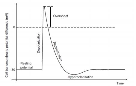
Figure 1. Schematic representation of an action potential in an excitable cell.

1.2. Activation of the Heart and the ECG

The contraction and relaxation of the heart muscles that enables the irrigation of all the circulatory system is adequately related with the action potential propagation in the heart. The electrical activity of the heart originates in the sino-atrial node. The impulse then rapidly spreads through the right atrium to the atrioventricular node. It also spreads through the atrial muscle directly from the right atrium to the left atrium. The electrical conduction system of the heart is composed of the following structures [4]:

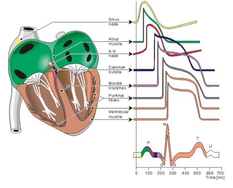
Figure 2. Propagation of the Action Potential through heart [5].

In ECG, P-wave is generated by activation of the muscle of both atria, result of atrial depolarization. The impulse travels very slowly through the AV node, then very quickly through the bundle of His, then the bundle branches, the Purkinje network, and finally the ventricular muscle. This generates the Q-wave. Next the left and right ventricular free walls, which form the bulk of the muscle of both ventricles, gets activated, with the endocardial surface being activated before the epicardial surface. This generates the R-wave. A few small areas of the ventricles are activated at a rather late stage. This generates the S-wave. Finally, the ventricular muscle repolarizes. This generates T-wave [6].

The activation sequence of the action potential in the heart leads to the production of closed-line action currents that flow in the thoracic volume conductor. Potentials measured at the outer surface (the body surface) are referred as Electro- cardiograms (ECGs). Electrocardiograph is generated with the help surface electrodes, electronic amplifiers and filters and display devices. It provides information about the heart rate, rhythm, and morphology.

FD is a descriptive measure that has been proven useful in quantifying the complexity or self-similarity of biomedical signals. ECG signal of a human heart is a self-similar object, so it must have a fractal dimension that can be extracted using mathematical methods to identifying and distinguish specific states of heart pathological conditions. Three different methods for computing FD values will be investigated from ECG time series signals depending on fractal geometry in order to extract its main features.

2. Methodology

Fractal Dimension is a descriptive measure that has been proven useful in quantifying the complexity or self-similarity of biomedical signals. ECG signal of a human heart is a self-similar object, so it must have a fractal dimension that can be extracted using mathematical methods to identifying and distinguish specific states of heart pathological conditions [7] [8]. In general, a fractal is defined as a set having non-integer dimension. Consequently, the fractal dimension (FD) is introduced as a factor highly correlated with the human perception of object’s roughness. FD fills the gap between one- and two-dimensional objects. The more complex the contour of the curve, the more it fills the plane and the more its fractal dimension will be closer to 2. This section investigates three different methods for computing FD values from ECG time series signals (RR intervals) depending on fractal geometry in order to extract its main features.

A. Relative Dispersion (RD) Method

B. Power Spectral Density (PSD) Method

C. Rescaled Range Method

2.1. Relative Dispersion (RD) Method

One-dimensional approach that can be applied to an isotropic signal of any dimension [9]. Making estimates of the variance of the signal at each of several different levels of resolution form the basis of the technique; for fractal signals a plot of the log of the standard deviation versus the log of the measuring element size (the measure of resolution) gives a straight line with a slope of 1 - D, where D is the fractal dimension. The characterizing Hurst coefficient, H is a measure of irregularity; the irregularity or anticorrelation in the signal is maximal at H near zero. White noise with zero correlation has H = 0.5. For one-dimensional series, H = 2 - D, where D is the fractal dimension, 1<D<2 [9].

There is a strong relationship between the measure of variation (the coefficient of variation) and the resolution of measurement. This is a simple one dimensional spatial analysis which we level as RD analysis, where RD is the relative dispersion i.e. the standard deviation divided by the mean. Mathematically it can be expressed as:

Standard Deviation =

Where, Random variable

= Mean of the variables

N = Number of Samples

H not equal to 0.5, the SD will be proportional to , n being the bin size or time resolution interval. By calculating the RD () for different bin sizes, n and fitting the square law function:

RD=RD₀ [9]

Where, RD₀ is the RD for some reference bin size no.

The exponent can be best estimated by a log-log transformation.

log(RD)=log(RD₀) +(H-1)log(n/n₀), Here H-1=slope [9]

ForFractal Dimension, D=2-H. So, D=1-slope. So, fractal dimension from this equation can easily be estimated. The fit is little improved when longer signals are used.

a) Analysis Procedure in Brief

1.  At first specified data (RR intervals of ECG signal) is divided into different series of Bin size.

2.  Then calculated Standard deviation and Mean for different Bin size of data.

Determine the arithmetic mean of data set by adding all of the individual values of the set together and dividing by the total number of values.

3.  Then standard deviation is normalized by dividing with the arithmetic mean, which yields the relative dispersion RD of the data series.

Table 1. FD Calculation for Normal ‘data 210’.

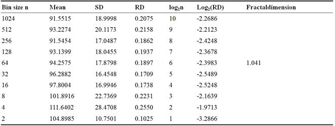
Table 2. FD Calculation for Abnormal ‘data106’.

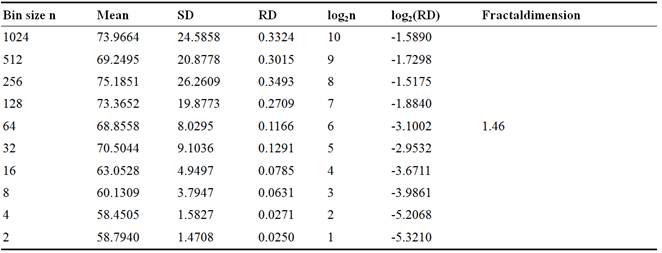
1.  The results are then plotted against log₂(n) versuslog₂(RD), where n is the bin size or the time resolution interval.

2.  The MATLAB function ‘polyfit()’ is used to fit a least square straight line over the log₂(n) versuslog₂(RD) curve.

Figure 3. Actual and approximated straight line for normal data.

Figure 4. Actual and approximated straight line for abnormal data.

The slope of the straight line is then used to calculate the fractal dimension: (D=1-slope)

Table 3. FD’s calculation for several Normal data.

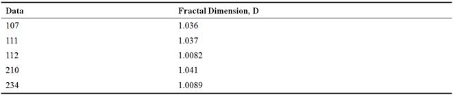
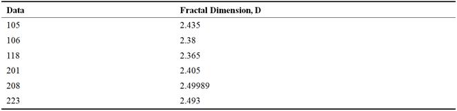
Table 4. FD’s calculation for several Abnormal data.

b)Comparison and Comments

Figure 5. FDs of Normal and Abnormal data of RD method.

From the figure it is clear that there is a difference in fractal dimension between normal and abnormal data. This difference varies mainly in the slope. If data is normal- SD will be small, so RD will be small and log₂(RD) also will be small. And when log₂(n) versus log₂(RD) is plotted Slope will be low.

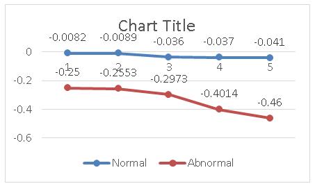
Figure 6. Ramp for normal and abnormal data.

In general, with the increase of data length, calculated fractal dimension in general, gets closer to the actual result.

We know, Standard Deviation =

For the case of Fractal dimensions,

For normal, Standard Deviation = 0.0162

For abnormal, Standard Deviation = 0.0936

It is seen that 2nd value of is more than 1st value. It is clear that 2^nd values are for abnormal because it is largely deviated from average. Relative Dispersion (RD) Analysis is well suited for long signals.

Figure 7. Flow Chart for Power Spectral Density Analysis.

2.2. Power Spectral Density Analysis

The power spectrum (the square of the amplitude from the Fourier transform) of an unpolluted fractional Brownian motion is known to be described by a power law function: |A|²= 1/ f ^β

Where |A| is the magnitude of the spectral density at frequency f, with an exponent equal to β = 2H + 1. In general, fractal signals always have such a very broad spectrum. When the derivative is taken from a fractal signal, β is reduced by two. Thus, for fractional Brownian noise, fBn, β is expected to be: β=2H+1.

Here again, a straight line is fitted from a log-log plot, and H is calculated from the slope β. Power spectrum method applies the power law variation of time series. A strong relationship exists between fractal dimension and power law index of time series. In the frequency domain, fractal time series exhibit power law properties:P(f) ~ f ^–α

Where P(f) is the power spectral density, f, and the exponent α is the so called power-spectral index. For the values region between FD=1 and FD =2 the following relationship between FD and α is valid: FD=(5-α)/2, for 1<FD<2

In other words, the fractal dimension of a time series can be calculated directly from its power spectrum.

a) Analysis Procedure in Brief

1.  At first simulated data is loaded.

2.  Power spectral density is estimated by using MATLAB function ‘PSD’ [10] [11].

Function Format: [Pxx,F]= psd(x,nfft,fs,window,noverlap)

It returns a vector of frequencies, the same size as Pxx at which the PSD is estimated. The PSD is plotted on log scale by using ‘log log’ command. The plots of the power spectral densities against the normalized frequency in the log scale are for normal and abnormal data assuming sampling frequency.

1.  Least-square straight line is then fitted over the PSD plotted.

Figure 8. PSD and approximated straight line for normal.

Figure 9. PSD and approximated straight line for abnormal.

2.  From the graphs, the ramp of the approximated straight line and fractal dimensions are calculated for different data series. For PSD method, Fractal dimension, D= (5-slope)/2

Table 5. FD’s for different normal data.

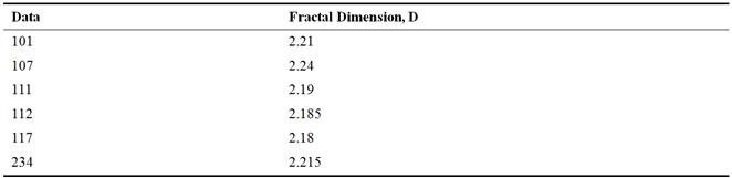
Table 6. FD’s for different abnormal data.

b) Comparison and Comments

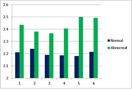
Figure 10. FDs are plotted for Normal and Abnormal data.

From the figure it is clear that there is a difference in Fractal Dimension between normal and abnormal data. This difference varies mainly in the slope.

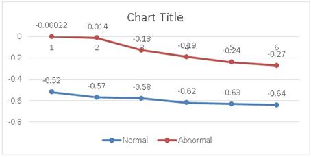
Figure 11. Ramp for Normal and Abnormal data.

2.3. Rescaled Range Analysis

Hurst (1965) developed the rescaled range analysis, a statistical method is used to analyze long records of natural phenomena. There are two factors used in this analysis: firstly, the range R, this is the difference between the minimum and maximum 'accumulated' values or cumulative sum of X(t,τ) of the natural phenomenon at discrete integer-valued time t over a time span τ (taw), and secondly the standard deviation S, estimated from the observed values Xi(t). Hurst found that the ratio R/S is very well described for a large number of natural phenomena by the following empirical relation [12-18]:

where τ is the time span, and H the Hurst exponent. The coefficient c was taken equal to 0.5 by Hurst. R and S are

–Min() for the range 1

And

The Relation between Hurst exponent and the fractal dimension is simply D=2-H. We calculate the individual calculations for each interval length. A straight line is fitted in the log-log plot: Log[R(T)/S(T)] = c + H log(T). Where H = slope. So, Fractal dimension, D= 2-H. With the help of this equation we can easily evaluate fractal dimension in rescaled range analysis[19].

a) Analysis Procedure in Brief

1.  At first specified data is divided into different series of Bin size.

2.  Then calculated standard deviation for different Bin size of data.

3.  Maximum and minimum of integral for each lag interval is then calculated to find out the range, R of each interval.

4.  Finally, the R/S ratio is calculated from the average of each slot R/S ratio.

Table 7. R/S analysis for Normal ‘data 107’.

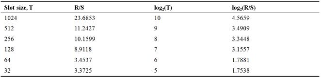
Table 8. R/S analysis for Abnormal ‘data 201’.

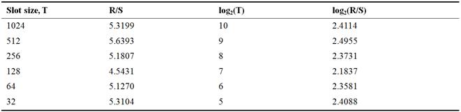
1.  The results are then plotted against log₂(t ) vs log₂(R/S), where tis the length of the time.

2.  The MATLAB function ‘polyfit()’ is used to fit a least square straight line over the log₂(t) vslog₂(R/S) curve.

Figure 12. Actual and approximated straight line for normal using R/S analysis.

Figure 13. Actual and approximated straight line for abnormal using R/S analysis.

From the above graphs, the slope of the straight line is then used to calculate the fractal dimension.

In the R/S analysis, fractal dimension D=2-H

Table 9. FD’s for different normal data by R/S analysis.

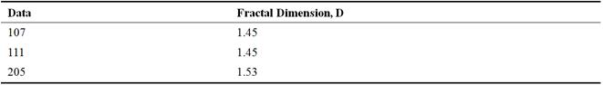
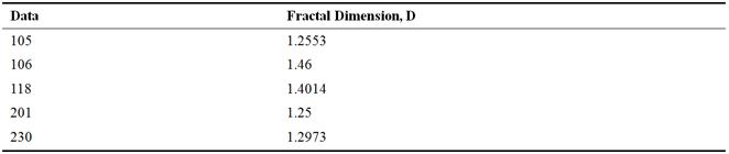
Table 10. FD’s for different abnormal data by R/S analysis.

b) Comparison and Comments

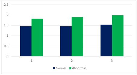
Figure 14. FDs are plotted for Normal and Abnormal data.

From the figure it is clear that there is a difference in fractal dimension between normal and abnormal data. This difference varies mainly in the slope.

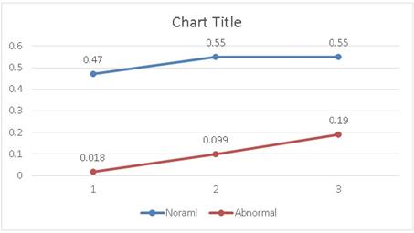
Figure 15. Difference in ramp for normal and abnormal data.

In Rescaled Range Analysis there is no linear variation of fractal dimension with data length or closely spaced data series.

For the case of Fractal dimensions,

For normal, Standard Deviation =0.001422

For abnormal, Standard Deviation = 0.004717

We see that 2^nd value of  is more than 1^st value. It is clear that 2^nd values are for abnormal because it is largely deviated from average.

3. Result and Discussion

In this research, fractal dimension for both normal and abnormal data are calculated and differences in fractal dimension between them for the case of three proposed methods are also calculated. From the calculated fractal dimension there is a sort of distance between normal and abnormal data that is cleared from the figure of ramp which have been plotted for normal and abnormal data. More distance will clear the more accuracy. Differences are not equal for all the three cases. In RD method under FD average value of normal data is 1.02622 and average value of abnormal data is 1.3328. It is observed that the range of difference is 30%. In PSD method under FD average value of normal data is 2.2033 and average value of abnormal data is 2.4296. It is observed that the range of difference is 22.63%. In R/S method under FD average value of normal data is 1.48 and average value of abnormal data is 1.8989. It is observed that the range of difference is 41.89%. One may find a quick hint from the fact that, in general, data series is suited better by R/S analysis rather than RD and PSD analysis. R/S analysis gives the more difference between normal and abnormal data. So it has a better accuracy to calculate fractal dimension than others.

4. Conclusions and Future Work

This paper aims to analysis heart rate variability (HRV) applying three different methods to calculate fractal dimension (FD) of instantaneous heart rate (IHR) derived from ECG. These non-linear techniques are applied to different raw data (RR intervals of ECG) that are derived from the sample ECG records from MIT-BIH database. The results found from this work are analyzed to see how they differ between normal and abnormal in the examined ECG record. There also has some classical technique to Heart rate analysis. In futureheart abnormalities will be detected by using several frequency domain methods such as cross entropy analysis, Support Vector Machine (SVM), Discrete Cosine Transform (DCT) and Wavelet Transform etc.

References

1. https://en.wikipedia.org/wiki/Electrocardiography
2. https://faculty.washington.edu/chudler/ap.html
3. http://hyperphysics.phy-astr.gsu.edu/hbase/biology/actpot.html
4. http://www.itaca.edu.es/cardiac-action-potential.htm
5. http://www.j-circ.or.jp/english/sessions/reports/64th-ss/nerbonne-l1.htm
6. http://www.bem.fi/book/06/06.htm
7. http://www.wahl.org/fe/HTML_version/link/FE4W/c4.htm
8. https://en.wikipedia.org/wiki/Fractal_dimension
9. http://www.ncbi.nlm.nih.gov/pmc/articles/PMC3459993/
10. http://www.mathworks.com/help/signal/ug/psd-estimate-using-fft.html
11. http://www.mathworks.com/help/matlab/examples/fft-for-spectral-analysis.html
12. Mandelbrot BB, Van Ness JW. Fractional brownian motions, fractional noises and applications.SIAM Rev. 1968;10:422–437.
13. Mandelbrot BB, Wallis JR. Noah, Joseph, and operational hydrology. Water Resour Res. 1968;4:909–918.
14. Mandelbrot BB, Wallis JR. Some long-run properties of geophysical records. Water Resour Res. 1969;5:321–340.
15. Mandelbrot BB, Wallis JR. Computer experiments with fractional Gaussian noises. Part 3, mathematical appendix. Water Resour Res. 1969;5:260–267.
16. Mandelbrot BB, Wallis JR. Robustness of the rescaled range R/S in the measurement of noncyclic long run statistical dependence. Water Resour Res. 1969;5:967–988.
17. Mandelbrot BB, Wallis JR. Computer experiments with fractional Gaussian noises. Part 2, rescaled ranges and spectra. Water Resour Res. 1969;5:242–259.
18. Hurst HE. Long-term storage capacity of reservoirs.Trans AmerSocCivEngrs. 1951;116:770–808.
19. Hurst HE, Black RP, Simaiki YM. Long-term Storage: An Experimental Study. Constable; London: 1965.

Biographical Notes