Breast Cancer Risk Detection Using Digital Infrared Thermal Images

Nader Abd El-Rahman Mohamed^*

Biomedical Engineering Department, Misr University for Science and Technology (MUST), Cairo, Egypt

Abstract

Early breast cancer detection, is one of the most important areas that researchers are working on, and it can increase the rate of diagnosis, cure and survival of the affected women. Considering the high cost of treatment as well as the high prevalence of the disease among women, early diagnosis will be the most significant step in reducing the health and social complications of this disease. Breast cancer is the major cause of cancer-related mortality among women worldwide. Early detection of cancer, especially breast cancer, will facilitate the treatment process. Cancer isranked as the 3rd cause of death. The aim was to develop an automatic breast cancer detection software that uses image processing techniques to analyze thermal breast images to detect the signs shown in these images for early detection of breast cancer. MATLAB was used as the programming environment. A new algorithm is proposed for the extraction of the breast characteristic features based on image analysis and image statistics. These features are extracted from the thermal image captured by a thermal camera. These features can be used to classify the breast either to be normal or suspected cancerous using a Neural Network classifier. The algorithm was tested with 206 breast images. Success rate of 96.12% is reached.

Keywords

Cancer Detection, Breast Thermal Image, Thermography, Image Analysis, Image Statistics

Received: August 23, 2015
Accepted: August 28, 2015
Published online: September 2, 2015

@ 2015 The Authors. Published by American Institute of Science. This Open Access article is under the CC BY-NC license. http://creativecommons.org/licenses/by-nc/4.0/

1. Introduction

Breast thermal image is a highly specialized form of medical imaging; it can’t be done with an ordinary camera. All objects with a temperature above absolute zero (−273 K) emit infrared radiation from their surface. The Stefan-Boltzmann Law defines the relation between radiated energy and temperature by stating that "The total radiation emitted by an object is directly proportional to the object’s area and emissivity and the fourth power of its absolute temperature". Since the emissivity of human skin is extremely high (within1% of that of a black body), measurements of infrared radiation emitted by the skin can be converted directly into accurate temperature values. This makes infrared imaging an ideal procedure to evaluate surface temperatures of the body.

Clinical infrared imaging is a procedure that detects, records, and produces an image of a patient’s skin surface temperatures and thermal patterns. The image produced resembles the likeness of the anatomic area under study. The procedure uses equipment that can provide both qualitative and quantitative representations of these temperature patterns.

Infrared imaging does not entail the use of ionizing radiation, venous access, or other invasive procedures; therefore, the examination poses no harm to the patient. Classified as a functional imaging technology, infrared imaging of the breast provides information on the normal and abnormal physiologic functioning of the sensory and sympathetic nervous systems, vascular system, and local inflammatory processes.

On January 29, 1982, the Food and Drug Administration published its approval and classification of thermography as an adjunctive diagnostic screening procedure for the detection of breast cancer. Since then, numerous medical centers and independent clinics have used thermography for a variety of diagnostic purposes.

As mentioned breast thermal image can’t be done with an ordinary camera and there are many important technical aspects to consider when choosing an appropriate clinical infrared imaging system, and in order to produce diagnostic quality infrared images, certain laboratory and patient preparation protocols must be strictly adhered to.

2. Methodology

2.1. Patient Preparation and Thermal Breast Image Data Acquisition

Infrared imaging must be performed in a controlled environment. The primary reason for this is the nature of human physiology. Changes from a different external (non-controlled room) environment, clothing, and the like, produce thermal artifacts. In order to properly prepare the patient for imaging, the patient should be instructed to refrain from sun exposure, stimulation or treatment of the breasts, cosmetics, lotions, antiperspirants, deodorants, exercise, and bathing before the exam.

The imaging room must be temperature and humidity-controlled and maintained between 18 and 23°C, and kept to within 1°C of change during the examination. This temperature range insures that the patient is not placed in an environment in which their physiology is stressed into a state of shivering or perspiring. The room should also be free from drafts and infrared sources of heat (i.e., sunlight and incandescent lighting). In keeping with a physiologically neutral temperature environment, the floor should be carpeted or the patient must wear shoes in order to prevent increased physiologic stress.

Lastly, the patient must undergo 15 min of waist-up nude acclimation in order to reach a condition in which the body is at thermal equilibrium with the environment. At this point, further changes in the surface temperatures of the body occur very slowly and uniformly; thus, not affecting changes in homologous anatomic regions. Thermal artifacts from clothing or the outside environment are also removed at this time. The last 5 min of this acclimation period is usually spent with the patient placing their hands on top of their head in order to facilitate an improved anatomic presentation of the breasts for imaging.

The captured breast thermal images were obtained using an infra-red camera FLIR SC-620 which is used to convert infrared radiation emitted from the skin surface into electrical impulses that are visualized in color on a monitor [1-4]. This visual image graphically maps the body temperature and is referred to as a thermo-gram. The spectrum of colors indicates an increase or decrease in the amount of infrared radiation being emitted from the body surface. Since there is a high degree of thermal symmetry in the normal body, subtle abnormal temperature asymmetry's can be easily identified.  Figure 1, shows the breast thermography procedure.

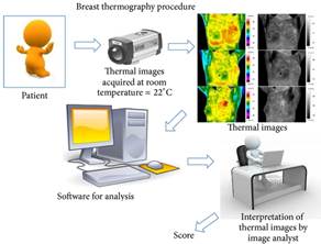
Figure 1. Breast Thermography Procedure.

The captured image is a 640x480x8 bits Digital color-mapped Infra-red Thermal Image (DITI), which is converted into 24-bit RGB image. Figure 2, shows an example.

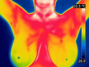
Figure 2. Breast Thermal Image.

2.2. RGB and HIS Color Models

The RGB color model (where R, G, and B are abbreviated from the colors Red, Green, and Blue respectively) is used, in this work, to display the color breast thermal image, while the HSI color model (where H, S, and I are abbreviations for Hue, Saturation, and Intensity respectively) is used in all processing stages. The RGB and HSI have an invertible relation between them [5].

Figure 3, shows the RGB color breast thermal image, and Figure 4, shows the intensity component (gray level image) of the HIS color model.

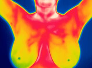
Figure 3. RGB Breast Thermal Image.

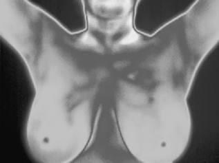
Figure 4. Breast Intensity Image.

2.3. Background Elimination

The optimum threshold technique [5] is applied to the gray level image, to make the pixels belonging to the body thermal image region and the pixels belonging to the background region separable. The optimum threshold is calculated using the following iterative algorithm:

1.   Assuming no knowledge about the exact location of thermal region, consider as a first approximation that the four corners of the image contain background pixels only, and the remainder contains thermal pixels.

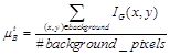
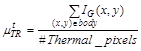
2.   At step t, compute  and  as the mean background and thermal gray level respectively, where segmentation into background and body at step t is defined by the threshold value  determined in the previous step.

                 (1)

                  (2)

where: I_G(x,y) is the intensity of the pixel (x,y) in the intensity  image.

1.   Set  which provides an updated background/thermal distinction.

2.   If  then halt; otherwise go to step (2). Where epson is a small number like one or two.

Figure 5, shows the histogram of the breast thermal images, which indicates that both background, and the thermal body region can be separable.

Figure 6, shows the result of the background elimination step after using the optimum thresholding technique.

The resultant image is used to mask the background in the thermal image. Figure 7, shows the breast thermal image after background elimination process.

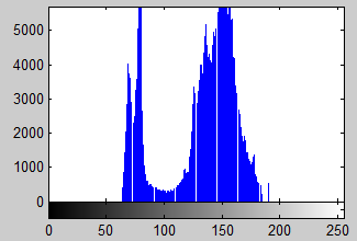
Figure 5. Histogram of the breast thermal image.

Figure 6. The result of the background elimination step.

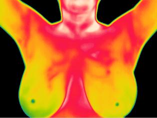
Figure 7. Breast Thermal Image after background elimination.

2.4. Region of Interest (ROI) Identification

In this step, thermal images are segmented and separated on left and right breast regions.

The proposed algorithm is based on tracking the body outline edge by applying a suitable edge detector such as Canny edge detector or Sobel edge detector on the mask image, then the algorithm is applied separately to both sides; right and left.

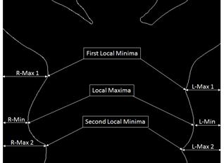
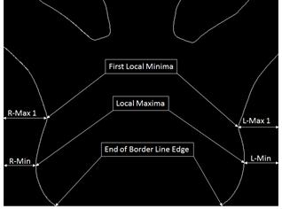
The proposed algorithm consists of three steps:

1.   Find the first minimum pixel location on the body outline edge in the thermal images, and to insure local minima, more than 10 pixel are taken and compared together to find the least minimum value.

2.   Continue with the body outline edge, and find the maximum pixel location.

3.   Then, continue with the body outline edge till finding the second minimum pixel location as in Figure 8(a), or reaching the end of the thermal image as in Figure 8(b).

Figure 8 illustrates the steps used to segment and separate the left and right breast regions (ROI).

(a)

(b)

Figure 8. Steps used to segment and separate the left and right breast regions (ROI).

Top, bottom, left and right boundaries are generated based on these points, as well as the middle line of the body, to separate the left and right breast regions.

Figure 9, shows the right breast region.

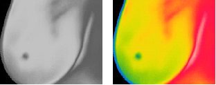
Figure 9. Right Breast Region.

Figure 10, shows the left breast region.

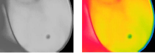
Figure 10. Left Breast Region.

2.5. Breast Contour Detection

In this stage, ROI undergoes further processing to accurately localizing the right and left breast masses. Breast mass contour detection algorithm is based on the generalized Hough transform.

The Hough transform is a technique, which can be used to isolate features of a particular shape within an image. Because it requires that the desired features be specified in some parametric form, the classical Hough transform is most commonly used for the detection of regular curves such as lines, circles, ellipses, etc. A generalized Hough transform can be employed in applications where a simple analytic description of features is not possible. The main advantage of the Hough transform technique is that it is tolerant of gaps in feature boundary descriptions and is relatively unaffected by image noise.

Many anatomical parts investigated in medical images contain feature boundaries which can be described by regular curves. For instance, breast boundaries in breast thermal image are parabola like shapes. The Hough transform can be generalized to detect shapes like parabolas.

The proposed algorithm uses Hough Transform to detect parabola in a binary image using the representation of parabola:

                                     (3)

Where

are the coordinates of the parabola vertex.

is the angle of the parabola in polar coordinates.

p is the distance between vertex and focus of parabola.

According to the Hough Transform, and the motivating idea behind the Hough technique for parabola detection is that each input pixel in image space corresponds to a parabola in Hough space and vice versa.

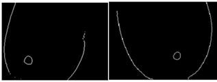
Figure 11. Right & Left Breast Contours.

The Generalized Hough transform to detect parabola is performed using the following algorithm:

1.   Run edge detection algorithm, such as the Canny edge detector, on subject image

2.   Input edge/boundary points into Hough Transform (Parabola detecting)

3.   Generate a curve for each point in Cartesian space (also called accumulator array)

4.   Extract local maxima from the accumulator array, for example using a relative threshold. In other words, we take only those local maxima in the accumulator array whose values are equal to or greater than some fixed percentage of the global maximum value.

5.   De-Houghing into Cartesian space yields a set of parabola descriptions of the image subject.

Figure 11, shows both right and left breast contours.

2.6. Image Analysis and Feature Vector

Image analysis is the term that is used to embody the idea of automatically extracting useful information from an image. The important point regarding image analysis is that this information is explicit and can be used in subsequent decision making processes. The grey-level histogram of an image often contains sufficient information to allow analysis of the image content, and in particular, to discriminate between objects and to distinguish objects with defects. It has the distinct advantage that it is not necessary to segment the image first and it is not dependent on the location of the object in the image. The analysis is based exclusively on the visual appearance of the image as a whole. There are two ways to consider histogram analysis:

1.   By extracting features which are descriptive of the shape of the histogram.

2.   By matching two histogram signatures.

In the former case, discrimination can be achieved using the classification techniques, where in the latter case, the template matching paradigm is more appropriate.

Color moments are measures that can be used to differentiate images based on their features of color. Once calculated, these moments provide a measurement for color similarity between images.

The basis of color moments lays in the assumption that the distribution of color in an image can be interpreted as a probability distribution. Probability distributions are characterized by a number of unique moments (e.g. Normal distributions are differentiated by their mean and variance). It therefore follows that if the color in an image follows a certain probability distribution, the moments of that distribution can then be used as features to identify that image based on color.

Color moments are scaling and rotation invariant. The first four color moments are used as features in image retrieval applications as most of the color distribution information is contained in the low-order moments. Since color moments encode both shape and color information they are a good feature to use under changing lighting conditions. Color moments can be computed for any color model. Four color moments are computed per channel (e.g. 12 moments if the color model is RGB or HIS and 16 moments if the color model is CMYK). Computing color moments is done in the same way as computing moments of a probability distribution.

A total of twelve statistical features "Color Moments" are frequently used as a means of describing the shape of histograms, and computing image features; Mean, Standard deviation, Skewness and Kurtosis.

Mean is the first color moment and can be interpreted as the average color in the image, and it can be calculated by using the following formula:

Mean:                           (4)

Standard deviation is the second color moment, which is obtained by taking the square root of the variance of the color distribution.

Variance:             (5)

Skewness is the third color moment. It measures how asymmetric the color distribution is, and thus it gives information about the shape of the color distribution. Skewness can be computed with the following formula:

Skewness:            (6)

Kurtosis is the fourth color moment, and, similarly to skewness, it provides information about the shape of the color distribution. More specifically, kurtosis is a measure of how flat or tall the distribution is in comparison to normal distribution, and it can be calculated by using the following formula:

Kurtosis:         (7)

2.7. Grey-Level Co-occurrence Matrices

Texture is "the variation of data at scales smaller than the scales of interest". Textures are generally pattern that we can percept from the surface of an object that helps us recognize what it is and to predict the properties that it has.

Texture classification has been a field that is frequently studied as it is applicable onto many applications, such as wood species identification, rock texture classification, and defects inspection. Since texture analysis techniques can be implemented in various machine learning problems, by studying the algorithms of texture classification, we can also implement them into other similar implementations involving texture-liked subjects such as text detection, face detection, retinal recognition and etc.

The importance of texture measure, is that it allows the system to be easily used in various environments and various locations, and allows the orientation of capturing such as the distance from lens to subject of interest and lightings to be controlled.

A statistical method of examining texture that considers the spatial relationship of pixels is the gray-level co-occurrence matrix (GLCM), also known as the gray-level spatial dependence matrix. The GLCM characterize the texture of an image by calculating how often pairs of pixel with specific values and in a specified spatial relationship occur in an image.

The gray-level co-occurrence matrix (GLCM) is created by calculating how often a pixel with the intensity (gray-level) value i occurs in a specific spatial relationship to a pixel with the value j. By default, the spatial relationship is defined as the pixel of interest and the pixel to its immediate right (horizontally adjacent), but you can specify other spatial relationships between the two pixels. Each element (i, j) in the resultant GLCM is simply the sum of the number of times that the pixel with value i occurred in the specified spatial relationship to a pixel with value j in the input image.

Figure 12, illustrates how the first three values in a GLCM are calculated. In the output GLCM, element (1, 1) contains the value 1 because there is only one instance in the input image where two horizontally adjacent pixels have the values 1 and 1, respectively. GLCM (1, 2) contains the value 2 because there are two instances where two horizontally adjacent pixels have the values 1 and 2. GLCM (1, 3) has the value 0 because there are no instances of two horizontally adjacent pixels with the values 1 and 3. Similarly, processing the rest of the input image, scanning the image for other pixel pairs (i, j) and recording the sums in the corresponding elements of the GLCM.

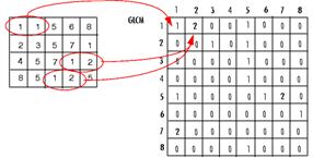
Figure 12. Gray Level Co-Occurrence Matrix (GLCM) Construction.

There are a total of twenty features (four directions are computed; horizontal, vertical, and two diagonal directions) that are commonly used [6-8]:

1.   "Contrast" is used to measure the local variations.

2.   "Energy" is also known as uniformity of Angular Second Moment (ASM) which is the sum of squared elements from the Grey-level Co-occurrence Matrices (GLCM).

3.   "Homogeneity" is alternatively called Inverse difference moment, which measures the distribution of elements in the GLCM with respect to the diagonal.

4.   "Entropy" measures the statistical randomness.

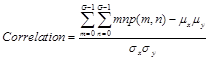
5.   "Correlation" shows the relation between inter-pixels.

                       (8)

          (9)

      (10)

             (11)

         (12)

where:

                     (13)

                     (14)

                (15)

                (16)

G is the grey level of the breast image.

p(m.n) is the Grey-level Co-occurrence Matrices (GLCM).

2.8. Feature Extraction and Classification Stage

In the feature extraction stage, a valid feature vector of thirty two features is extracted from ROI image to represent the breast mass characteristic features. This feature vector is passed to the Neural Network (NN) Classifier, which is the final stage.

Figure 13, shows how the breast mass characteristic features are fed to the Neural Network Classifier.

Neural networks have seen an explosion of interest over the last few years and are being successfully applied across an extraordinary range of problem domains, in areas as medicine, engineering, geology and physics. There are two main reasons for NN investigation, first is to try to get an understanding on how human brain function and second is desire to build machines that are capable for solving complex problems that sequentially operating computers were unable to solve.

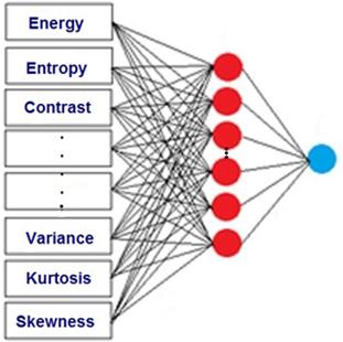
Figure 13. Artificial Neural Network.

The workflow for the general neural network design process has seven primary steps:

1.   Collect data

2.   Create the network

3.   Configure the network

4.   Initialize the weights and biases

5.   Train the network

6.   Validate the network (post-training analysis)

7.   Use the network

Choosing number of nodes for each layer will depend on problem NN is trying to solve, types of data network is dealing with, quality of data and some other parameters. Number of input and output nodes depends on training set in hand.

If there are too many nodes in hidden layer, number of possible computations that algorithm has to deal with increases. Picking just few nodes in hidden layer can prevent the algorithm of its learning ability. The way to control NN is by setting and adjusting weights between nodes [9-10].

One of the most popular Neural Network algorithms is back propagation algorithm, which consists of four main steps:

1.   Feed-forward computation.

2.   Back propagation to the output layer.

3.   Back propagation to the hidden layer.

4.   Weight updates.

Initial weights are usually set at some random numbers and then they are adjusted during NN training. After choosing the weights of the network randomly, the back propagation algorithm is used to compute the necessary corrections. During the NN training weights are updated after iterations. If results of NN after weights updates are better than previous set of weights, the new values of weights are kept and iteration goes on. The algorithm stops when the value of the error function has become sufficiently small.

Figure 14, shows the Artificial Neural Network training phase.

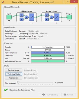
Figure 14. Artificial Neural Network Training Phase.

3. Results & Discussion

A total of 206 thermography images of the breast (187 normal and 19 abnormal patterns) were analyzed. A feature vector of thirty two features representing the breast mass characteristics is determined.

1. Twelve statistical features "Color Moments"; Mean, Standard deviation, Skewness and Kurtosis for each color space; Hue, Saturation, and Intensity (4 x 3 = 12).

2. Twenty texture features "Texture Measures"; Contrast, Energy, Homogeneity, Entropy and Correlation in the four directions; horizontal, vertical, and two diagonal directions of the Grey-level Co-occurrence Matrices (5 x 4 =20).

The classifier employed in this research was the feed forward back propagation neural network classifier which consists of: 32 input layers, 15 hidden layers, and 1 output layer.

Breast thermo-grams were classified into positive thermo-grams containing masses and negative thermo-grams containing normal tissues.

Figure 15, shows the neural network training performance, reaching Mean Squared Error of 0.1005.

Figure 16, shows the neural network training state, and Figure 17, shows the neural network training regression.

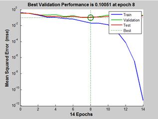
Figure 15. Artificial Neural Network Training Performance.

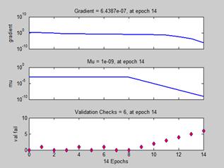
Figure 16. Artificial Neural Network Training State.

Finally, the performance in recognition can be evaluated by the following factors: Accuracy (number of samples correctly classified), Sensitivity (proportion of positive cases that are well detected), and Specificity (proportion of negative cases that are well detected). They are defined as follows:

    (17)

                 (18)

                  (19)

where,

TP is the number of true positives.

FP is the number of false positives.

TN is the number of true negatives.

FN is the number of false negatives.

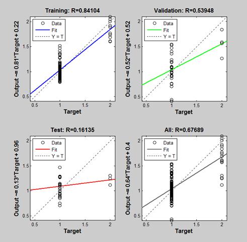
Figure 17. Artificial Neural Network Training Regression.

Another evaluation parameter is the Precision or Positive Predictive Value (proportion of positive results in classification are true positive results) and Negative Predictive Value (proportions of negative results in classification that are true negative results), and they are expressed mathematically as:

              (20)

              (21)

Results indicated that classification results are promising, with Accuracy ratio of 96.12%, Sensitivity of 78.95%, Specificity of 97.86%, Positive Predictive Value of 78.95%, and Negative Predictive Value of 97.86%.

4. Conclusion

This paper develops a computer-aided approach for automating analysis of breast thermo-grams. This kind of approach will help the diagnostics as a useful second opinion. The use of Thermal Infra-Red images for breast cancer detection was showing promising classification results. Experimental results show that feature extraction is a valuable approach to extract the signatures of breast characteristics. This kind of diagnostic aid, especially in a diseases like breast cancer where the reason for the occurrence is not totally known, will reduce the false positive diagnosis rate and increase the survival rate among the patients since the early diagnosis of the disease is more curable than in a later stage.

References

1. Silva, L. F., Saade, D. C. M., Sequeiros-Olivera, G. O., Silva, A. C., Paiva, A. C., Bravo, R. S. andConci, A., "A New Database for Breast Research with Infrared Image", Journal of Medical Imaging and Health Informatics, Volume 4, Number 1, March 2014 , pp. 92-100.
2. Watmough DJ. The role of thermographic imaging in breast screening, discussion by CR Hill. In Medical Images: Formation, Perception and Measurement, 7^thLH Gray Conference: Medical Images, pp. 142-58, 1976.
3. Keyserlingk JR, Ahlgren PD, Yu E, Belliveau N andYassa M. "Functional infrared imaging of the breast", IEEE EngineeringinMedicine and Biology, 19(3), pp. 30-41. 2000.
4. Gautherie M., Atlas of breast thermography with specific guidelines for examination andinterpretation. Milan, Italy: PAPUSA. 1989.
5. R. C. Gonzalez and R. E. Woods, Digital Image Processing. Second Edition, Prentice Hall, New Jersy, 2002.
6. A. Baraldi, and F. Parmiggiani, "An investigation of the textural characteristics associated with gray level co-occurrence matrix statistical parameters", IEEE Transactions on Geoscience and Remote Sensing, Vol. 33, No. 2, pp. 293-304, 1995.
7. M. Partio, B. Cramariuc, M. Gabboui, and A. Visa, "Rock Texture Retrieval using Gray Level Co-occurrence Matrix", Proceedings of 5th Nordic Signal Processing Symposium, 2002.
8. M. Tuceryan, and A. K. Jain, "Texture Analysis, The Handbook of Pattern Recognition and Computer Vision, Ed. 2", World Scientific Publishing Co., 1998.
9. Statsoft, Model Extremely Complex Functions, Neural Networks, http://www.statsoft.com/textbook/neural-networks/ apps (accessed 25 January 2015).
10. Berndt Müller, Joachim Reinhardt, Michael T. Strickland, Neural Networks: An Introduction (Physics of Neural Networks) 2nd Edition, Springer-Verlag, 1995.