
International Journal of Bioinformatics and Biomedical Engineering, Vol. 1, No. 2, September 2015 Publish Date: Aug. 24, 2015 Pages: 153-161
A Study on Discrete Model of Three Species Syn Eco System with Unlimited Resources for the Second Species
Department of Mathematics, Chaitanya Degree College (Autonomous), Hanamkonda, Telangana State, India
Abstract
In this paper, the three species syn eco-system comprises of a commensal (S1), two hosts S2 and S3 ie., S2 and S3 both benefit S1, without getting themselves effected either positively or adversely. Further S2 is a commensal of S3, S3 is a host of both S1, S2 and the second species has unlimited resources. The basic equations for this model constitute as three first order non-linear coupled ordinary difference equations. All possible equilibrium points are identified based on the model equations at two stages and criteria for their stability are discussed. Further the numerical solutions are computed for specific values of the various parameters and the initial conditions.
Keywords
Commensal, Equilibrium Point, Host, Oscillatory, Stable, Unstable
Received: July 7, 2015
Accepted: August 8, 2015
Published online: August 24, 2015
@ 2015 The Authors. Published by American Institute of Science. This Open Access article is under the CC BY-NC license. http://creativecommons.org/licenses/by-nc/4.0/
Contents
1. Introduction 2. Basic Equations of the Model 2.1. Notation Adopted 2.2. Basic Equations 3. Equilibrium States 3.1. One Period Equilibrium States 3.2. The Stability Analysis of One Period Equilibrium States 3.3. Two Period Equilibrium States 3.4. The Stability Analysis of Two Period Equilibrium States 4. Numerical Examples 5. Discussion and Conclusions Acknowledgment
1. Introduction
Ecology, a branch evolutionary biology, deals with living species that coexist in a physical environment sustain themselves on common resources. It is a common observations that the species of same nature can not flourish is isolation without any interaction with species of different kinds. Significant researches in the area of theoretical ecology have been discussed by Kot [1] and by [2]. Several ecologists and mathematicians contributed to the growth of this area of knowledge. Mathematical ecology can be broadly divided into two main sub-divisions, Autecology and Synecology, which are described in the treatises of Arumugam [3], Sharma [4]. Syn-ecology is an ecosystem comprised of two or more distinct species. Species interact with each other in one way or other. The Ecological interactions can be classified as Ammensalism, Competition, Commensalism, Neutralism, Mutualism, Predation, Parasitism and so on.
Mathematical Modeling plays a vital role in providing insight into the mutual relationships (positive, negative) between the interacting species. The general concepts of Modeling in Biological Science have been initiated by several authors Ma [5], Murray [6], and Sze-Bi Hsu [7]. Recently the authors Papa Rao et al. [8], Shivareddy et al. [9], Srinivas [10] and Kumar et al. [11] discussed three species ecological models such as predation, completion and commensalism. Srinivas [12] studied the competitive ecosystem of two species and three species with limited and unlimited resources. Later, Narayan et al. [13] studied prey-predator ecological models with partial cover for the prey and alternate food for the predator. Acharyulu et al. [14,15] derived some productive results on various mathematical models of ecological Ammensalism with multifarious resources in the manifold directions. Further, Kumar [16] studied some mathematical models of ecological commensalism. The present author Prasad [17-22] investigated continuous and discrete models on the three species syn-ecosystems.
The present investigation is on an analytical study of a typical three species (S1, S2, S3) syn-eco system. The system comprises of a commensal (S1), two hosts S2 and S3 ie, S2 and S3 both benefit S1, without getting themselves effected either positively or adversely. Further S2 is a commensal of S3 and S3 is a host of both S1, S2. Commensalism is a symbiotic interaction between two populations where one population (S1) gets benefit from (S2) while the other (S2) is neither harmed nor benefited due to the interaction with (S1). The benefited species (S1) is called the commensal and the other, the helping one (S2) is called the host species. A common example is an animal using a tree for shelter-tree (host) does not get any benefit from the animal (commensal). Some more real-life examples of commensalism are, i. The clownfish shelters among the tentacles of the sea anemone, while the sea anemone is not affected. ii. A flatworm attached to the horse crab and eating the crab’s food, while the crab is not put to any disadvantage. iii. Sucker fish (echeneis) gets attached to the under surface of sharks by its sucker. This provides easy transport for new feeding grounds and also food pieces falling from the sharks prey, to Echeneis.
2. Basic Equations of the Model
2.1. Notation Adopted
Ni(t) : The population strength of Si at time t, i = 1,2,3; t: Time instant ; ai: Natural growth rate of Si , i = 1, 2, 3; aii: Self inhibition coefficients of Si, i = 1, 3; a12, a13: Interaction coefficients of S1 due to S2 and S1 due to S3; a23 : Interaction coefficient of S2 due to S3. Further the variables N1, N2, N3 are non-negative and the model parameters a1, a2, a3, a11, a12, a33, a13, a23 are assumed to be non-negative constants.
2.2. Basic Equations
Consider the growth of the species during the time interval![]() .
.
![]() (1)
(1)
![]() (2)
(2)
![]() (3)
(3)
The equations (1), (2) and (3) can be written in the nonlinear autonomous system of discrete equations as
![]() (4)
(4)
![]() (5)
(5)
![]() (6)
(6)
where ![]() .
.
3. Equilibrium States
The equilibrium states for a discrete model are defined in terms of the period of no growth. i.e, ![]()
![]() where r is the period of the equilibrium state.
where r is the period of the equilibrium state.
3.1. One Period Equilibrium States
![]() .
.
The system under investigation has five equilibrium states given by
![]()
![]()
![]()
![]()
![]()
![]()
![]()
3.2. The Stability Analysis of One Period Equilibrium States
3.2.1. The Stability of E1
![]() , where r is an integer and i = 1, 2, 3.
, where r is an integer and i = 1, 2, 3.
Hence, E1 (0, 0, 0) is stable.
3.2.2. The Stability of E2
![]()
where r is an integer and i = 1, 2.
Hence, E2 is stable.
3.2.3. The Stability of E3
![]()
where r is an integer and i = 2, 3.
Hence, E3 is stable.
3.2.4. The Stability of E4

Hence, E4 is stable.
3.2.5. The Stability of E5
![]()
where r is an integer.
Hence, E5 is stable.
At this stage all the five equilibrium states are stable.
3.3. Two Period Equilibrium States
![]()
The system under investigation has twenty five equilibrium states given by
![]()
![]() .
.


![]()
The states E3 and E4 coincide when α3 = 3 and do not exist when α3 < 3.
![]() .
.


![]()
The states E7and E8 coincide when α1 = 3 and do not exist when α1 < 3.
![]()
![]()


![]()
The states E11and E12 coincide when β1 = 3 and do not exist when β1 < 3.

![]()


The states E15 and E16 coincide when γ1 = 3 and do not exist when γ 1 < 3.

![]()


The states E19 and E20 coincide when µ1 = 3 and do not exist when µ1 < 3.
![]()
![]()


![]()
The states E23 and E24 coincide when δ1 = 3 and do not exist when δ 1 < 3.
3.4. The Stability Analysis of Two Period Equilibrium States
The equilibrium states E1, E2 and E6 are stable as established in 3.2. Now we will discuss the stability of other equilibrium states except these three states.
3.4.1. The Stability of E3
![]() , where r is an integer and i = 1, 2.
, where r is an integer and i = 1, 2.
![]()
![]()
where r is an integer.
Hence, E3 oscillates between
![]() ,
,
when α3 > 3and is stable when α3 = 3.
3.4.2. The Stability of E4
![]() , where r is an integer and i = 1, 2.
, where r is an integer and i = 1, 2.
![]()
![]()
where r is an integer.
Hence, E4 oscillates between
![]() ,
,
when α3 > 3and is stable when α3 = 3.
3.4.3. The Stability of E5
![]()
where r is an integer and i = 1, 2.
Hence, E5 is stable.
3.4.4. The Stability of E7
![]()
![]()
where r is an integer.
![]() , where r is an integer and i = 2, 3.
, where r is an integer and i = 2, 3.
Hence, E7 oscillates between
![]() ,
,
when α1 > 3and is stable when α1 = 3.
3.4.5. The Stability of E8
![]()
![]()
where r is an integer.
![]() , where r is an integer and i = 2, 3.
, where r is an integer and i = 2, 3.
Hence, E8 oscillates between
![]() ,
,
when α1 > 3and is stable when α1 = 3.
3.4.6. The Stability of E9
![]()
where r is an integer and i = 2, 3.
Hence, E9 is stable.
3.4.7. The Stability of E10
![]()
where ![]() is an integer.
is an integer.
Hence, E10 is stable.
3.4.8. The Stability of E11
![]()
![]()
![]() where r is an integer.
where r is an integer.
Hence, E11 oscillates between
![]() ,
,
when β1 > 3and is stable when β1 = 3.
3.4.9. The Stability of E12
![]()
![]()
![]() where r is an integer.
where r is an integer.
Hence, E12 oscillates between
![]() ,
,
when β1 > 3and is stable when β1 = 3.
3.4.10. The Stability of E13
![]()
where r is an integer.
Hence, E13 is stable.
3.4.11. The Stability of E14
![]() where
where ![]() is an integer except 0 and 1
is an integer except 0 and 1
![]()
![]()
![]()
where ![]() is an integer.
is an integer.
Hence, E14 is unstable, when α3 > 3and is stable when α3 = 3.
3.4.12. The Stability of E15
![]()
where ![]() is an integer except 0 and 1
is an integer except 0 and 1
![]()
![]()
![]()
where ![]() is an integer.
is an integer.
Hence, E15 is unstable, when α3 > 3and is oscillatory when α3 = 3.
3.4.13. The Stability of E16
![]()
where ![]() is an integer except 0 and 1.
is an integer except 0 and 1.
![]()
![]()
![]()
where ![]() is an integer.
is an integer.
Hence, E16 is unstable, when α3 > 3and is oscillatory when α3 = 3.
3.4.14. The Stability of E17
![]() where
where ![]() is an integer except 0 and 1
is an integer except 0 and 1
![]()
![]()
![]()
where ![]() is an integer.
is an integer.
Hence, E17 is unstable, when α3 > 3and is stable when α3 = 3.
3.4.15. The Stability of E18
![]() where
where ![]() is an integer except 0 and 1.
is an integer except 0 and 1.
![]()
![]()
![]()
where ![]() is an integer.
is an integer.
Hence, E14 is unstable, when α3 > 3and is stable when α3 = 3.
3.4.16. The Stability of E19
![]()
where ![]() is an integer except 0 and 1.
is an integer except 0 and 1.
![]()
![]()
![]()
where ![]() is an integer.
is an integer.
Hence, E19 is unstable, when α3 > 3and is oscillatory when α3 = 3.
3.4.17. The Stability of E20
![]()
where ![]() is an integer except 0 and 1.
is an integer except 0 and 1.
![]()
![]()
![]()
where ![]() is an integer.
is an integer.
Hence, E20 is unstable, when α3 > 3and is oscillatory when α3 = 3.
3.4.18. The Stability of E21
![]() where
where ![]() is an integer except 0 and 1.
is an integer except 0 and 1.
![]()
![]()
![]()
where ![]() is an integer.
is an integer.
Hence, E21 is unstable, when α3 > 3and is stable when α3 = 3.
3.4.19. The Stability of E22
![]()
where ![]() is an integer.
is an integer.
Hence, E22 is stable.
3.4.20. The Stability of E23
![]()
![]()
![]()
where r is an integer.
Hence, E23 oscillates between
![]() ,
,
when δ1 > 3and is stable when δ1 = 3.
3.4.21. The Stability of E24
![]()
![]()
![]()
where r is an integer.
Hence, E24 oscillates between
![]() ,
,
when δ1 > 3and is stable when δ1 = 3.
3.4.22. The Stability of E25
![]()
where ![]() is an integer.
is an integer.
Hence, E25 is stable, when δ3 = 3and α3 = 3.
At this stage, in all twenty five equilibrium states, only the nine states E1, E2, E5, E6, E9,E10, E13, E22, E25 are stable and E3, E4, E7, E8, E11, E12, E23, E24 are oscillatory and remaining all are unstable.
4. Numerical Examples
![]()
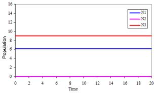
Figure 1. Variation of population against time for a1 = 1.5, a11 = 1, a13 = 0.4, a2 = 1.05, a22 = 3.4, a23 = 4.53, a3 = 2.7, a33 = 0.3, N1(0) = 6.1, N2(0) = 0, N3(0) = 9.
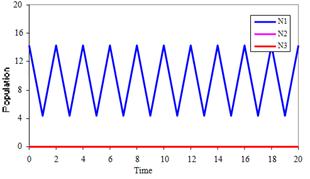
Figure 2. Variation of population against time for a1 = 3.6, a11 = 0.3, a13 = 2.6, a2 = 4.7, a22 = 1.28, a23 = 3.33, a3 = 1.23, a33 = 2.1, N1(0) = 14.32, N2(0) = 0, N3(0) = 0.
The numerical solutions of the discrete model equations computed for specific values of the various parameters and the initial conditions. The results are illustrated in Figures 1 to 4.
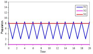
Figure 3. Variation of population against time for a1 = 1.5, a11 = 1.2, a13 = 0.4, a2 = 2.11, a22 = 1.4, a23 = 0.50, a3 = 1.6, a33 = 0.2, N1(0) = 8.6, N2(0) = 0, N3(0) = 8.
Figure 4. Variation of population against time for a1 = 2.6, a11 = 1.29, a13 = 0.01, a2 = 0.7, a22 = 1.53, a23 = 0.85, a3 = 3.6, a33 = 0.3, N1(0) = 2.1, N2(0) = 0, N3(0) = 14.32.
5. Discussion and Conclusions
The present paper deals with an investigation on a discrete model of three species syn eco-system with unlimited resources for the second species. The system comprises of a commensal (S1) common to two hosts S2 and S3 ie., S2 and S3 both benefit S1, without getting themselves effected either positively or adversely. Further S2 is a commensal of S3, S3 is a host of both S1, S2. All possible equilibrium points of the model are identified based on the model equations at two stages.
Stage-I: Ni (t + 1) = Ni (t); i = 1, 2, 3.
Stage-II: Ni (t + 2) = Ni (t); i = 1, 2, 3.
In Stage-I there are only five equilibrium points, while the Stage-II there would be twenty five equilibrium points. All the five equilibrium points in Stage-I are found to be stable while in stage-II only nine are stable. Further the numerical solutions for the discrete model equations are computed.
Acknowledgment
I thank to Professor (Retd), N.Ch. Pattabhi Ramacharyulu, Department of Mathematics, National Institute of Technology, Warangal (T.S.), India for his valuable suggestions and encouragement.
References
- Kot, M. (2001), Elements of Mathematical Ecology, Cambridge University Press, UK.
- Gillman, M. (2009), An Introduction to Mathematical Models in Ecology and Evolution, Wiley-Blackwell, UK.
- Arumugam, N. (2006), Concepts of Ecology, Saras Publication, India.
- Sharma, P.D. (2009), Ecology and Environment, Rastogi Publications, India.
- Ma, Z. (1996), The Study of Biology Model, Anhui Education Press, China.
- Murray, J.D. (1993), Mathematical Biology, Springer, New York.
- Sze-Bi Hsu. (2004), Mathematical Modeling in Biological Science, Tsing-Hua University, Taiwan.
- Papa Rao, A.V.,Narayan, K.L. and Bathul, S. (2012), A Three Species Ecological Model with a Pray, Predator and a Competitor to both the Prey and Predator, International Journal of Mathematics and Scientific Computing, 2(1), 70 - 75.
- Shivareddy, K., Pattabhiramacharyulu, N.Ch. (2011), A Three Species Ecosystem Comprising of Two Predators Competing for a Prey, Advances in Applied Science Research, 2(3), 208 - 218.
- Srinivas, M.N. (2011), A Study of Bionomic Harvesting for a Three Species Ecosystem Consisting of Two Neutral Predators and a Prey, International Journal of Engineering Science and Technology, 3(10), 7491 - 7496.
- Kumar, N.P., Pattabhiramacharyulu, N.Ch. (2010), A Three Species Ecosystem Consisting of a Prey, Predator and a Host Commensal to the Prey, Int. J. Open Problems Compt. Math., 3(1), 92 - 113.
- Srinivas, N.C. (1991), Some Mathematical Aspects of Modeling in Bio-medical Sciences, Kakatiya University, Ph.D Thesis.
- Narayan, K.L., Pattabhiramacharyulu, N.Ch. (2007), A Prey-Predator Model with Cover for Prey and Alternate Food for the Predator and Time Delay, Int. Journal of Scientific Computing, 1, 7 - 14.
- Acharyulu, K.V.L.N., Pattabhiramacharyulu, N.Ch. (2010), An Enemy- Ammensal Species Pair With Limited Resources –A Numerical Study, Int. Journal Open Problems Compt. Math., 3,339-356.
- Acharyulu, K.V.L.N., Pattabhiramacharyulu, N.Ch. (2011), An Ammensal-Prey with three species Ecosystem, International Journal of Computational Cognition , 9, 30 - 39.
- Kumar, N.P. (2010), Some Mathematical Models of Ecological Commensalism, Acharya Nagarjuna University, Ph.D. Thesis.
- Prasad, B.H. (2014), The Stability Analysis of a Three Species Syn-Eco-System with Mortality Rates. Contemporary Mathematics and Statistics, 2, 76-89.
- Prasad, B.H. (2014), A Study on DiscreteModelofThreeSpeciesSyn-Eco-System with Limited Resources. Int. JournalModern Education and Computer Science,11, 38-44.
- Prasad, B.H. (2014), A Discrete Model of a Typical Three Species Syn- Eco – System with Unlimited Resources for the First and Third Species. Asian Academic Research Journal of Multidisciplinary, 1, 36-46.
- Prasad, B.H. (2015), A Study on the Discrete Model of Three Species Syn-Eco-System with Unlimited Resources. Journal of Applied Mathematics and Computational Mechanics, 14, 85-93.
- Prasad, B.H. (2015), On the Stability of a Three Species Syn-Eco-System with Mortality Rate for the Third Species. Applications and Applied Mathematics: An International Journal, 10, 521-535.
- Prasad, B.H. (2015), A Study on Discrete Model of a Typical Three Species Syn-Ecology with Limited Resources.InternationalJournalofAnimal Biology, 1, 69-73.


