
Agricultural and Biological Sciences Journal, Vol. 1, No. 2, April 2015 Publish Date: Apr. 8, 2015 Pages: 62-70
Assessing Climate Suitability for Sustainable Vegetable Roselle (Hibiscus sabdariffa var. sabdariffa L.) Cultivation in India Using MaxEnt Model
Medagam Thirupathi Reddy1, *, Hameedunnisa Begum1, Neelam Sunil2, Someswara Rao Pandravada2, Natarajan Sivaraj2
1Vegetable Research Station, Dr. Y. S. R. Horticultural University, Rajendranagar, Hyderabad, Telangana, India
2National Bureau of Plant Genetic Resources, Regional Station, Rajendranagar, Hyderabad, Telangana, India
Abstract
Vegetable Roselle (Hibiscus sabdariffa var. sabdariffa L.) is a tropical leafy vegetable sparsely under cultivation in India. The idea was to use crop modeling in identifying the most suitable areas for vegetable Roselle cultivation in India. Dataset for vegetable Roselle presence locations (n=23 points) was generated from two surveys organized by National Bureau of Plant Genetic Resources, Regional Station, Rajendranagar in collaboration with Vegetable Research Station, Rajendranagar in parts of Andhra Pradesh and Odisha states, India during 2010-11. WorldClim dataset representing current climatic conditions was downloaded from http://www.worldclim.org. Vegetable Roselle presence locations dataset and WorldClim dataset were used with Maximum entropy (MaxEnt) modeling to generate the climate suitability map to show potential vegetable Roselle sites in India. The MaxEnt model performed better than random (random prediction AUC = 0.500) with an average AUC value of 0.993 and 0.992 for training and test data, respectively. We classified climatic zones in terms of their suitability for vegetable Roselle cultivation, based on the existence probability determined using the MaxEnt model. The results show that the MaxEnt model can be used to study the climatic suitability for vegetable Roselle cultivation. This approach can be used in other countries as well that lack precise coordinates of vegetable Roselle cultivation occurrences and generate a preliminary map of potential areas because it may be too late to wait for the precise coordinates of crop occurrences to generate a perfect climate suitability map.
Keywords
Area Under Receiver Operating Characteristic (ROC) Curve (AUC), Climate Suitability Map, DIVA-GIS, MaxEnt Model, Presence-Only Data, Thresholds
Received: March 16, 2015
Accepted: March 29, 2015
Published online: April 6, 2015
@ 2015 The Authors. Published by American Institute of Science. This Open Access article is under the CC BY-NC license. http://creativecommons.org/licenses/by-nc/4.0/
1. Introduction
Vegetable Roselle (Hibiscus sabdariffa var. sabdariffa L.), a member of the Malvaceae family, is known in different countries by various common names, including Roselle, razelle, sorrel, red sorrel, Jamaican sorrel, Indian sorrel, Guinea sorrel, sour-sour, Queensland jelly plant, Jamaican sorrel, red sorrel, rozelle hemp, natal sorrel,rosella, rohzelu, sabdriqa, lalambarilal-ambari, patwa, laalambaar (Morton, 1987; Mahadevan et al., 2009; Kays, 2011). It is an annual erect, bushy, herbaceous shrub (Berhaut, 1979), probably native from India to Malaysia. Roselle was introduced to the other parts of the world such as West Indies, Central America and Africa (Purseglove, 1968; Morton, 1987) where it best grown in tropical and sub-tropical regions (Fasoyiro et al., 2005). It is now widely cultivated throughout the tropics and subtropics especially in Sudan, China, Thailand, Egypt, Mexico, and the West India (Purseglove, 1974; El-Saidy et al., 1992), the Indian subcontinent, parts of Asia, America, Australia and Africa (Cobley, 1968). It is cultivated in various parts of Punjab, Uttar Pradesh, Andhra Pradesh, Assam, Bihar, Madhya Pradesh, Maharashtra, Orissa and West Bengal in India (Mahadevan et al., 2009). It is a famous leafy vegetable crop with several uses and benefits (Ottai et al., 2006). Roselle plays an important role in providing nutritional and health security and income generation and subsistence among rural farmers in developing countries (Cisse et al., 2009). There is need for vegetable Roselle production to be increased to meet demand. Vegetable Roselle production can be increased either by bringing the new areas under commercial cultivation or by improving the productivity of Roselle cultivars in traditional growing areas.
The concept of sustainable agriculture involves producing quality products in an environmentally benign, socially acceptable, and economically acceptable way (Addeo et al., 2001). In order to comply with these principles of sustainable agriculture, the crops are to be grown where they suit best which require a thorough environmental suitability analysis. Environmental suitability is an important aspect that has direct impact on the productivity of the crop and a prerequisite for sustainable agricultural production. An important component in this is crop modeling. Various modeling tools are used to support the decision-making and planning in sustainable agriculture. As vegetable Roselle is an important crop in India, it is essential to find out the areas of suitability for vegetable Roselle cultivation. Site suitability is an important factor to determine the productivity of the crop (Parthasarthy et al., 2007). Suitability maps are useful to determine areas which will have the greatest success for growing a particular crop (Parthasarthy et al., 2007). Several site suitability models have been used extensively to evaluate the potential impact of climate change on shifts in the production and growing regions of various crops (Easterling et al., 1993; Rosenzweig et al., 1995; Tubiello et al., 2000; Tubiello et al., 2002). Crop prediction models include EcoCrop (EC), Maximum Entropy (MaxEnt), Crop Niche Selection in Tropical Agriculture (CaNaSTA) and Decision Support System for Agrotechnology Transfer (DSSAT). These are the most appropriate models to use in the assessment of suitability of various areas for crop cultivation.
Of the above models, MaxEnt is the most adapted model to use when presence-only data is available. We chose MaxEnt model because this is based on algorithms and represents a variety of different statistical approaches. Several articles describe its use in ecological modeling and explain the various parameters and measures involved (Phillips et al., 2004; Phillips et al., 2006; Elith et al., 2011). MaxEnt is considered as the most accurate model performing extremely well in predicting occurrences in relation to other common approaches (Hijmans and Graham, 2006), especially with incomplete information (Phillips et al., 2006). MaxEnt has been successfully used by many researchers earlier to predict distributions such as stony corals (Tittensor et al., 2009), macrofungi (Wollan et al., 2008), seaweeds (Verbruggen et al., 2009), forests (Carnaval and Moritz, 2008), rare plants (Williams et al., 2009) and many other species. MaxEnt is the most adapted model to use for coffee and mango (Eitzinger et al., 2013). Several methodologies have been used for model accuracy assessment in species distribution modeling. The area under receiver operating characteristic (ROC) curve (AUC) (Hanley and McNeil, 1982) and defined thresholds are the important tools used for the evaluation of MaxEnt model quality. Yet recent reviews revealed that neither crop modeling approaches nor the simulation tools are fully up to the task.
Use of MaxEnt model to assess climate suitability of vegetable Roselle for identifying the potential regions in Indian and/or world climate is the primary objective of the study.
2. Materials and Methods
2.1. Data Collection
2.1.1. Crop Presence Data of Vegetable Roselle
Crop presence data of vegetable Roselle was generated following random sampling strategy through two exploration surveys from 23 points covering four districts of Andhra Pradesh and one of Odisha (formerly Orissa), India by National Bureau of Plant Genetic Resources, Regional Station, Rajendranagar in collaboration with Vegetable Research Station, Dr. Y. S. R. Horticultural University, Rajendranagar during 2010-11. The geographical coordinates (longitude and latitude) of occurrence locations of vegetable Roselle were recorded using a Global Positioning System (Garmin GPS-12) Receiver. A total of 23 distributional localities (n=23 presence records) of vegetable Roselle were compiled into a database to generate a preliminary global and Indian national level climate suitability maps for vegetable Roselle cultivation using MaxEnt and/or DIVA-GIS, thus making use of the best available crop presence data (Table 1).
Table 1. Crop presence data of vegetable Roselle (Hibiscus sabdariffa var. sabdariffa L.) used in MaxEnt analysis
| S. No. | Crop presence point | S. No. | Crop presence point | ||
| Latitude (°N) | Longitude (°E) | Latitude (°N) | Longitude (°E) | ||
| 1 | 18.54223 | 84.02493 | 13 | 18.54108 | 83.32698 |
| 2 | 19.28835 | 84.40203 | 14 | 18.58578 | 83.36567 |
| 3 | 19.15080 | 84.25807 | 15 | 18.49613 | 83.27852 |
| 4 | 18.98718 | 84.02670 | 16 | 16.06700 | 78.90037 |
| 5 | 18.99768 | 84.04610 | 17 | 15.80077 | 78.21700 |
| 6 | 19.00472 | 84.07580 | 18 | 15.81733 | 78.05043 |
| 7 | 18.76913 | 84.40862 | 19 | 15.70093 | 78.08340 |
| 8 | 18.65385 | 84.30410 | 20 | 14.68413 | 77.65093 |
| 9 | 18.35955 | 82.89013 | 21 | 14.23387 | 77.60088 |
| 10 | 18.57197 | 83.79703 | 22 | 14.25098 | 77.68365 |
| 11 | 18.31328 | 83.57062 | 23 | 13.81762 | 77.50002 |
| 12 | 18.46287 | 83.31428 | |||
2.1.2. Climatological Data
Bioclimatic variables (BC) are often used in ecological niche modeling and they represent annual trends, seasonality and extreme or limiting environmental factors. For the current climate (baseline) of India, monthly data from the WorldClim database (Hijmans et al., 2005) sourced from global weather stations publicly and freely available and downloadable from www.worldclim.org. were used.
2.2. Data Analysis Using MaxEnt Model
A set of crop presence data of vegetable Roselle generated and a set of climatological data collected were used for training and testing for MaxEnt analysis using MaxEnt software version 3.3.3e (Phillips et al., 2006). Default settings were used in MaxEnt so that the complexity of the model varied depending upon the number of data points used for model fitting. Twenty five percentage of the entire set of presence records (n=23) constitute the test data. The remaining 75 percentage of the entire set of presence records (n=23) constitute the training data. The test points (test data) are a random sample taken from the species presence localities. The information available about the target distribution of vegetable Roselle often presents itself as a set of real-valued variables, called ‘features’, and the constraints are that the expected value of each feature should match its empirical average. The program starts with a uniform probability distribution and works in cycles adjusting the probabilities to maximum entropy. It iteratively alters one weight at a time to maximize the likelihood of reaching the optimum probability distribution. The probability distribution of vegetable Roselle is the sum of each weighted variable divided by a scaling constant to ensure that the probability value ranges from 0 to 1. The ASCI file generated by the MaxEnt run for vegetable Roselle occurrence points was imported to grid file using DIVA-GIS software version 7.5 (Hijmans et al., 2012). The grid layer generated was overlaid on India shape file using DIVA-GIS and analysed (Sundar and Mitsuko, 2005). The outcome is a crop probability map of vegetable Roselle.
2.3. Evaluation of MaxEnt Model
The area under receiver operating characteristic curve and defined thresholds were the tools used for the evaluation of quality of MaxEnt model in this study. The AUC and thresholds were generated from the same test and training data using MaxEnt software version 3.3.3e (Phillips et al., 2006).
3. Results and Discussion
3.1. Climate Suitability Maps of Vegetable Roselle
The basis for this project is the general notion that knowledge about environmental conditions at locations where particular plant species are successfully grown should provide a basis for summarizing crop growth parameters throughout the region. Plant species occurrence is not only defined however by climate variables, and exclusion of other important variables may reduce the ability to assess the required environmental growing conditions (Stanton et al., 2011). Climatic variables are the principal drivers of geographic distribution (Walker and Cocks, 1991; Guisan and Zimmerman, 2000). The distribution of vegetable Roselle cultivation depends on not only climate, socio-economic conditions, and local production technologies, but also on soil type, geographic characteristics, crop varieties, human activity, and so on. In this study, we considered the effects of climatic variables.
3.1.1. Analysis of Global Climate Suitability Map of Vegetable Roselle Generated Using MaxEnt Model
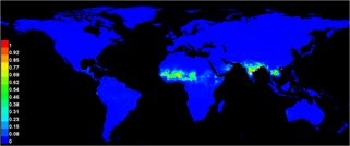
Figure 1. The preliminary global geographical distribution map of vegetable Roselle generated using MaxEnt model
The global climate suitability for vegetable Roselle cultivation using MaxEnt model is depicted in Figure 1. White dots show the presence locations used for training, while violet dots show test locations. Warmer colors show areas with better-predicted conditions. The red color indicates areas with a high probability of occurrence for vegetable Roselle, the blue and green represent moderately high probability of occurrence, the yellow color represents low probability of occurrence and the white indicates areas not suitable for vegetable Roselle. In fact, this global climate suitability map can be used in the countries that lack precise coordinates of vegetable Roselle occurrences and generate a preliminary climate suitability map of vegetable Roselle because it may be too late to wait for the precise coordinates of vegetable Roselle occurrences to generate a perfect climate suitability map.
3.1.2. Analysis of State-Wise Indian National Level Climate Suitability Map of Vegetable Roselle Generated Using MaxEnt Model and DIVA-GIS
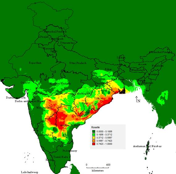
Figure 2. State-wise Indian national level climate suitability map of vegetable Roselle generated using MaxEnt software and DIVA-GIS
State-wise Indian national level climate suitability map for vegetable Roselle was generated using MaxEnt software and DIVA-GIS (Figure 2). Climatic zones were classified in terms of their suitability for vegetable Roselle cultivation, based on the existence probability determined using the MaxEnt model. The geographical ranges of climate suitability were depicted with different colors. The geographical ranges of the excellent area-red color (0.7087-1.0000), optimum area-orange color (0.5315-0.7087), suitable area-yellow color (0.3543-0.5315), less suitable area-light green color (0.1772-0.3543) and unsuitable area-green color (0.0000-0.1772) are shown in the climate suitability map of vegetable Roselle (Figure 2).
The excellent area in this study is slightly southward and eastward and it includes most parts of Andhra Pradesh, Karnataka, Maharashtra, Chhattisgarh, Odisha and West Bengal. These states had the potential regions for introducing and cultivating the vegetable Roselle on commercial scale. Hence, in these regions vegetable Roselle may be popularized in view of its potential. In addition, these states had the potential for planning in-situ on-farm conservation sites for vegetable Roselle landraces in the light of climate change scenario. Further, most of the western regions had ‘less suitable’and ‘unsuitable areas’, the northern parts of India had wholly ‘unsuitable’ area and the central parts of India had ‘less suitable’ area. We conclude that MaxEnt model is powerful first-cut tool for estimating relative site suitability across geographic regions in which candidate vegetable Roselle can be grown.
3.2. Evaluation of Quality of MaxEnt Model
Model utility is dependent on an evaluation of performance. This is a critical element of model-building. As with any modeling approach, the fit or accuracy of the model should be tested to determine the relevance of the model. The utility of MaxEnt in real world applications requires the knowledge of the model’s accuracy. The first step in evaluating the model produced by the two algorithms was to verify that both performed significantly better than random. For this purpose, we first used a threshold-dependent binomial test based on omission and predicted area. However, it does not allow for comparisons between algorithms, as the significance of the test is highly dependent on predicted area. The threshold-independent receiver operating characteristic analysis was used to characterize the performance of model at all possible thresholds by a single number, the area under the receiver operating characteristic curve, which may be then compared between algorithms.
3.2.1. The Area Under the Receiver Operating Characteristic Curve
A binomial test of omission (known areas of presence predicted absent) can be used to test whether or not the difference is significant (Phillips et al., 2006), and provides some information on the usefulness of the model. The ‘25’ we entered for ‘random test percentage’ command the program to randomly set aside 25% of the sample records for testing. This allows the program to do some simple statistical analysis. Much of the analysis used the use of a threshold to make a binary prediction, with suitable conditions predicted above the threshold and unsuitable below. The following picture (Figure3) shows the omission rate and predicted area as a function of the cumulative threshold. The omission rate is calculated both on the training presence records and on the test records. The omission rate should be close to the predicted omission, because of the definition of the cumulative threshold. Figure 3 shows how testing and training omission and predicted area vary with the choice of cumulative threshold. The omission on test samples (sky blue line) is a very good match to the predicted omission rate (black line), and the omission rate for test data drawn from the MaxEnt distribution itself. The predicted omission rate is a straight line (black line), by definition of the cumulative output format. In some situations, the test omission line (sky blue line) lies well below the predicted omission line (black line), while in some other situations the test omission line (sky blue line) lies well above the predicted omission line (black line): a common reason is that the test and training data are not independent, for example if they derive from the same spatially auto-correlated presence data. MaxEnt model was significantly better than random in binomial test of omission and predicted area curve. Because we have only occurrence data and no absence data, ‘fractional predicted area’ (the fraction of the total study area predicted present) is used instead of the more standard commission rate (fraction of absences predicted present).
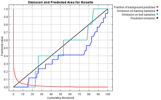
Figure 3. Graph generated by MaxEnt software showing omission and predicted area for vegetable Roselle
The threshold-independent indices used in or introduced to the species distribution models (SDMs) field include the area under the receiver operating characteristic curve. In the context of SDMs, the AUC of a model is equivalent to the probability that the model will rank a randomly chosen species presence site higher than a randomly chosen absence site (Pearce and Ferrier, 2000). To use the AUC without instances of absence, the ROC plot has to be modified so that instead of plotting Se against (1-Sp), it is plotted against the proportion of the background locations predicted as presences (or the proportionate area predicted as presence) for all possible thresholds (Phillips et al., 2006; Peterson et al., 2008). AUC’s are developed from ROC plots to provide a ranked approach for assessing differences in species distributions for developed models compared to a random distribution. AUC is currently considered to be the standard method to assess the accuracy of predictive distribution models. AUC of ROC is one of the most widely used accuracy measures in various disciplines including ecology (Lobo et al., 2008). Since its first proposal as an appropriate method to estimate the accuracy of species distribution models (Fielding and Bell, 1997), many studies have recommended its use in this field of research (Pearce and Ferrier, 2000; Manel et al., 2001; McPherson et al., 2004). The models are still ranked according to their AUC, i.e. the higher the better (Phillips et al., 2006). AUC has received some criticism (Lobo et al., 2008). AUC has been criticized by some researchers as it can give a misleading picture of model performance since it covers parts of the prediction range that is of no practical use (Briggs and Zaretzki, 2008). AUC is a misleading measure of the performance of predictive distribution models (Lobo et al., 2008).
Figure 4 shows the receiver operating curve for both training and test data. The area under the ROC curve is also given in Figure 4. In general, the specificity is defined using predicted area rather than true commission, which implies that the maximum achievable AUC is less than 1. If test data is drawn from the MaxEnt distribution itself, then the maximum possible test AUC would be 0.981 rather than 1; in practice the test AUC may exceed this bound. AUC designates the predictive accuracy of the model. The higher the AUC value the more accurate the predictions of the constructed model (Elith, 2002). In general, the value of AUC ranges from 0.5 and 1.0, indicating the following degrees of predictive accuracy: >0.90 = very good; AUC: 0.70-0.90 = good, AUC: <0.70 = uninformative (Swets, 1988). When the values of AUC are more than 0.75, the constructed model is applicable. In the present study, the AUC of the constructed model based on the potential climatic factors affecting the distribution of the vegetable Roselle cultivation zone was 0.993 for training data and 0.992 for test data. As we split data into two partitions, one for training and one for testing, it is quite normal for the training data (red line) to show a higher AUC (0.993) than the test data (blue line) with AUC of 0.992. The AUC was almost higher, indicating better discrimination of suitable versus unsuitable areas for the species. This value indicated that the constructed model had ‘very good’ predictive accuracy, and therefore, that it was highly suitable for predicting the geographic distribution of vegetable Roselle cultivation in India.
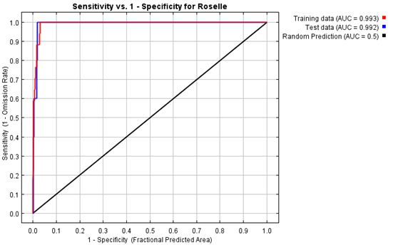
Figure 4. Graph generated by MaxEnt software showing receiver operating curve (ROC) for vegetable Roselle
Red line generated by using different thresholds. AUC of >0.5 denotes higher predictive power, AUC of 0.5 denotes random chance and AUC of <0.5 denotes worse than random. The red (training) line shows the ‘fit’ of the model to the training data. The blue (testing) line indicates the fit of the model to the testing data, and is the real test of the models predictive power. The turquoise (random prediction) line (black line) shows the line that you would expect if the model was no better than random. If the blue line (the test line) falls below the turquoise line then this indicates that the model performs worse than a random model would. The further towards the top left of the graph that the blue line is, the better the model is at predicting the presences contained in the test sample of the data. It is important to note that AUC values tend to be higher for species with narrow ranges, relative to the study area described by the environmental data. This does not necessarily mean that the model is better; instead this behaviour is an artifact of the AUC statistic. MaxEnt model was significantly better than random in receiver operating characteristic analysis.
3.2.2. Thresholds
The second approach used for MaxEnt model evaluation in this study was the defined thresholds. This approach involves selecting thresholds to establish sites that are considered suitable or unsuitable for the species of interest. Once a threshold has been identified, locations can be classified as suitable or unsuitable for the species of interest. These thresholds are established by maximizing sensitivity while minimizing specificity (Fielding and Bell, 1997; Phillips et al., 2006). Threshold values differ for each model and are selected to provide a desired balance between omission and commission (Fielding and Bell, 1997; Hernandez et al., 2006). Where this threshold is applied is determined from ROC plots and is selected at the discretion of the modeller. For example, when dealing with endangered species, the modeller may want to maintain zero omission error while identifying the minimum predicted area. However, if the modeller is interested in identifying any possible area that a species might use, then they would want to minimize commission error (Pearson et al., 2007).
Some common thresholds and corresponding omission rates are as follows (Table 2). Since test data are available, binomial probabilities were not calculated exactly as the number of test samples is less than 25. Hence, a normal approximation to the binomial was used. These are 1-sided p-values for the null hypothesis that test points are predicted no better than by a random prediction with the same fractional predicted area. The balance threshold minimises 6* training omission rate + 0.04* cumulative threshold + 1.60* fractional predicted area.
4. Conclusion
Fortunately, the crop presence data of vegetable Roselle collected through surveys provides a reliable and sound basis for the climate suitability analysis using MaxEnt software. Based on MaxEnt model, most suitable regions for vegetable Roselle species cultivation state-wise in India are identified and our understanding of vegetable Roselle species spread was enhanced. The MaxEnt model performed better than random with an average AUC value of 0.993 and 0.992 for training and test data, respectively. The results indicated good performance by MaxEnt model in predicting landscape distribution for vegetable Roselle. Results will be useful for designing local, regional and national-level planning for vegetable Roselle-based farming systems in India. This approach can be used in other countries that lack precise coordinates of vegetable Roselle occurrences and generate a preliminary map of potential areas because it may be too late to wait for the precise coordinates of crop occurrences to generate a perfect climate suitability map.
Table 2. Common thresholds and corresponding omission rates for the threshold-dependent binomial tests of omission
| Cumulative threshold | Logistic threshold | Description | Fractional predicted area | Training omission rate | Test omission rate | P-value |
| 1.000 | 0.006 | Fixed cumulative value 1 | 0.182 | 0.000 | 0.000 | 2.018E-4 |
| 5.000 | 0.031 | Fixed cumulative value 5 | 0.074 | 0.000 | 0.000 | 2.2E-6 |
| 10.000 | 0.081 | Fixed cumulative value 10 | 0.044 | 0.000 | 0.000 | 1.654E-7 |
| 15.403 | 0.141 | Minimum training presence | 0.029 | 0.000 | 0.000 | 2.178E-8 |
| 16.174 | 0.151 | 10 percentile training presence | 0.028 | 0.059 | 0.000 | 1.676E-8 |
| 15.403 | 0.141 | Equal training sensitivity and specificity | 0.029 | 0.000 | 0.000 | 2.178E-8 |
| 15.403 | 0.141 | Maximum training sensitivity plus specificity | 0.029 | 0.000 | 0.000 | 2.178E-8 |
| 23.057 | 0.244 | Equal test sensitivity and specificity | 0.019 | 0.118 | 0.000 | 2.267E-9 |
| 23.057 | 0.244 | Maximum test sensitivity plus specificity | 0.019 | 0.118 | 0.000 | 2.267E-9 |
| 2.952 | 0.013 | Balance training omission, predicted area and threshold value | 0.107 | 0.000 | 0.000 | 1.43E-5 |
| 13.661 | 0.125 | Equate entropy of thresholded and original distributions | 0.033 | 0.000 | 0.000 | 4.06E-8 |
Acknowledgement
The senior author is highly grateful to the National Bureau of Plant Genetic Resources, Regional Station, Rajendranagar, Hyderabad for sharing the crop presence data of vegetable Roselle with the Vegetable Research Station, Dr. Y. S. R. Horticultural University, Rajendranagar.
References
- Addeo, G., Guastadisegni, G. and Pisante, N. 2001. Land and water quality for sustainable and precision farming. Proceedings of the 1st World Congress on Sustainable Agriculture, Madrid, 1-4.
- Berhaut,J.1979. Floreillustree du Senegal. Tome VI: linaceesetnympheacees. Direction des Eauxet Forets, Dakar (Senegal), 635 p.
- Briggs,W.M.andZaretzki, R. 2008. The skill plot: a graphical technique for evaluating continuous diagnostic tests. Biometrics. 63, 250-261.
- Carnaval,A.C. and Moritz,C. 2008. Historical climate modeling predicts patterns of current biodiversity in the Brazilian Atlantic forest. Journal of Biogeography. 35, 1187-1201.
- Cisse,M., Dornier,M., Sakho,M., Ndiaye,A., Reynes,M. and Sock,O. 2009.The bissap (Hibiscus sabdariffa L.): composition and principal uses.Fruits. 64(3), 179-193.
- Cobley,L.S. 1968. An Introduction to Botany of Tropical Crops, Longman, London, pp. 95-98.
- Easterling,W.E., Crosson,P.R., Rosenberg,N.J., McKenny,M.S., Katz,L.A. and Lemon,K.M. 1993. Agricultural impacts and responses to climate-change in the Missouri-Iowas-Nebraska-Kansas (MINK) region. Climate Change. 24, 23-61.
- Eitzinger,A., Laderach,P., Carmona,S., Navarro,C.andCollet,L. 2013. Prediction of the impact of climate change on coffee and mango growing areas in Haiti. Full Technical Report, Centro Internacional de Agricultura Tropical (CIAT), Cali, Colombia.
- Elith, J. 2002. Quantitative methods for modeling species habitat: Comparative performance and an application to Australian plants. In Quantitative Methods for Conservation Biology, S. Fersonand M.Burgman, editors, New York, Springer, pp. 39-58.
- Elith,J., Phillips,S.J., Hastie,T., Dudik,M., Chee,Y.E. and Yates,C.J. 2011. A statistical explanation of MaxEnt for ecologists.Diversity and Distributions. 17, 43‐57.
- El-Saidy,S.M., Ismail,I.A.andEL-Zoghbi,M. 1992. A study on roselle extraction as a beverage or as a source for anthocyanins. Zagazig Journal of Agricultural Research. 19, 831-839.
- Fasoyiro,S.B., Ashaye,O.A., Adeola,A. and Samuel,F.O. 2005. Chemical and storability of fruits flavored (Hibiscus sabdariffa) drinks. World Journal of Agricultural Science. 1, 165-168.
- Fielding,A.H.andBell,J.F. 1997. A review of methods for the assessment of prediction errors in conservation presence/ absence models. Environmental Conservation. 24,38-49.
- Guisan,A. and Zimmerman,N. 2000. Predictive habitat distribution models in ecology. Ecological Modelling. 135, 147-186.
- Hanley,J.A.andMcNeil,B.J. 1982. The meaning and use of the area under a Receiver Operating Characteristic (ROC) curve. Radiology. 143, 29-36.
- Hernandez, P.A., Graham, C.H., Master, L.L. and Albert, D.L. 2006. The effect of sample size and species characteristics on performance of different species distribution modeling methods. Ecography. 29, 773-785.
- Hijmans,R.J., Cameron,S.E., Parra,J.L., Jones,P.G. and Jarvis,A. 2005. Very high resolution interpolated climate surfaces for global land areas. International Journal of Climatology. 25(15), 1965-1978.
- Hijmans, R.J. and Graham C. 2006. The ability of climate envelope models to predict the effect of climate change on species distributions.Global Change Biology.12, 2272-2281.
- Hijmans, R.J., Guarino, L.andMathur, P. 2012. DIVA-GIS Version 7.5, Manual. Available at: www.diva-gis.org.
- Kays, S.J. 2011. Cultivated vegetables of the world: A multilingual onomasticon. University of Georgia, Wageningen Academic Publishers, the Netherlands, 184 p.
- Lobo,J.M., Jimenez-Valverde,A.andReal,R. 2008. AUC: a misleading measure of the performance of predictive distribution models. Global Ecology and Biogeography. 17, 145-151.
- Mahadevan,N., Shivali and Kamboj,P. 2009. Hibiscus sabdariffa Linn. An overview. Natural Product Radiance. 8(1), 77-83.
- Manel,S., Williams,H.C.andOrmerod,S.J. 2001. Evaluating presence-absence models in ecology: the need to account for prevalence. Journal of Applied Ecology. 38, 921-931.
- McPherson J.M., Jetz W.andRogers, D.J. 2004. The effects of species’ range sizes on the accuracy of distribution models: ecological phenomenon or statistical artefact?. Journal of Applied Ecology. 41, 811-823.
- Morton, F.J. 1987. Roselle (Hibiscus sabdariffa L.). In Fruits of Warm Climates, C.F. Dowling Jr, editor, Creative Resources Systems, Inc. Miami, Florida.
- Ottai,M.E.S., Aboud,K.A., Mahmoud,I.M. and El-Hariri,D.M. 2006. Stability analysis of roselle cultivars (Hibiscus sabdariffa L.) under different nitrogen fertilizer environments. World Journal of Agricultural Science. 2(3), 333-339.
- Parthasarthy,U., Johny,A.K., Jayarajan,K. and Parthasarthy,V.A. 2007. Site suitability for turmeric production in India, a GIS interpretation. Natural Product Radiance. 6(2), 142-147.
- Pearce,J.andFerrier,S. 2000. Evaluating the predictive performance of habitat models developed using logistic regression. Ecological Modelling. 133, 225-245.
- Pearson, R.G., Raxworthy, C.J., Nakamura, M. and Peterson, A.T. 2007. Predicting species distributions from small numbers of occurrence records: a test case using cryptic geckos in Madagascar. Journal of Biogeography. 34(1), 102-117.
- Peterson,A.T., Papes,M.andSoberon,J. 2008. Rethinking receiver operating characteristic analysis applications in ecological niche modelling. Ecological Modelling. 213, 63-72.
- Phillips,S.J., Anderson,R.P. and Schapire,R.E. 2006. Maximum entropy modeling of species geographic distributions.Ecological Modelling.190, 231-259.
- Phillips,S.J., Dudik,M. and Schapire,R.E. 2004. A maximum entropy approach to species distribution modeling. Proceedings of the 21stInternational Conference on Machine Learning, Banff, Canada, 655-662.
- Purseglove,J.W.1968. Tropical crops: Dicotyledons, Longman Scientific and Technical Press, Harlow, England, 719 p.
- Purseglove, J.W. 1974. Tropical crops dicotyledons. Volume1 and 2, Longman Group Ltd., London, pp. 370-372.
- Rosenzweig,C., Allen Jr,L.H., Harper,L.A., Hollinger,S.E. and Jones,J.W. 1995. Climate change and Agriculture: Analysis of Potential International Impacts. ASA Special Publication Number 59, American Society of Agronomy Inc., Madison, WI.
- Stanton,J.C., Pearson,R.G., Horning,N., Ersts,P. and Akcakaya,H.R. 2011. Combining static and dynamic variables in species distribution models under climate change.Methods in Ecology and Evolution.3, 349-357.
- Sundar,S.S. and Mitsuko,C. 2005. A geographical information system for the analysis of biodiversity data. Gis Resource Document [WWW document]. URL http://www.pop.psu.edu/gia-core/pdfs/gis_rd_02-27.pdf
- Swets,J.A. 1988. Measuring the accuracy of diagnostic systems. Science. 240, 1285-1293.
- Tittensor, D.P., Baco, A.R., Brewin, P.E., Clark, M.R., Consalvey, M., Hall-Spencer, J., Rowden, A.A., Schlacher, T., Stocks, K.I.andRogers, A.D. 2009. Predicting global habitat suitability for stony corals on seamounts.Journal of Biogeography.36, 1111-1128.
- Tubiello,F.N., Donatelli,M., Rosenzweig,C. and Stockle,C.O. 2000. Effects of climate change and elevated Co2 on cropping systems: model predictions at two Italian locations. European Journal ofAgronomy. 13, 179-189.
- Tubiello,F.N., Donatelli,M., Rosenzweig,C. and Stockle,C.O. 2002. Effects of climate change on US crop production: simulation results using two different GCM scenarios. Part 1: Wheat, potato, maize and citrus. Climate Research. 20, 256-270.
- Verbruggen, H., Tyberghein, L., Pauly, K., Vlaeminck, C., Van Nieuwenhuyze, K., Kooistra, W., Leliaert, F.andDe Clerck, O. 2009. Macroecology meets macroevolution: evolutionary niche dynamics in the seaweed Halimeda.Global Ecology and Biogeography.18, 393-405.
- Walker,P. and Cocks,K. 1991. Habitat: a procedure for modeling a disjoint environmental envelope for a plant or animal species. Global Ecology and BiogeographyLetters. 1, 108-118.
- Williams, J.N., Seo, C.W., Thorne, J., Nelson, J.K., Erwin, S., O’Brien, J.M.andSchwartz, M.W. 2009. Using species distribution models to predict new occurrences for rare plants.Diversity and Distributions.15, 565-576.
- Wollan, A.K., Bakkestuen, V., Kauserud, H., Gulden, G.andHalvorsen, R.2008. Modelling and predicting fungal distribution patterns using herbarium data.Journal of Biogeography.35, 2298-2310.


