
International Journal of Life Science and Engineering, Vol. 1, No. 4, September 2015 Publish Date: Jul. 9, 2015 Pages: 165-170
Modelling Monthly Ugandan Shilling/US Dollar Exchange Rates by Seasonal Box-Jenkins Techniques
Ette Harrison Etuk1, *, Bazinzi Natamba2
1Department of Mathematics and Computer Science, Rivers State University of Science and Technology, Port Harcourt, Nigeria
2Department of Accounting, Faculty of Commerce, Makerere University Business School, Kampala, Uganda
Abstract
A brief history of the exchange rates between the Uganda shilling and the United States dollars is given. Moreover, this work involves modeling of their monthly exchange rates by seasonal Box-Jenkins methods. Clearly with time more shillings are exchanged for the dollar, an evidence of relative depreciation of the shilling. An inspection of a realization of the time series which covers from July 1990 to November 2014 reveals a 12-monthly seasonality. A 12-monthly seasonal differencing and then a non-seasonal differencing of the seasonal differences is enough to rid the series of non-stationarity. The autocorrelation structure of the resultant series suggests two seasonal autoregressive integrated moving average (SARIMA) models of orders: (0, 1, 1)x(0, 1, 1)12 and (0, 1, 1)x(1, 1, 1)12. Diagnostic checking shows that the former is the more adequate on all counts. It is therefore recommended that forecasting of the series be based on it.
Keywords
Uganda Shilling, Us Dollar, Foreign Exchange Rates, Sarima Models, Seasonal Models
Received: May 9, 2015
Accepted: June 3, 2015
Published online: July 7, 2015
@ 2015 The Authors. Published by American Institute of Science. This Open Access article is under the CC BY-NC license. http://creativecommons.org/licenses/by-nc/4.0/
1. Introduction
Despite the fact that many studies on inflation (Durevall et al. 2012) have tried to suggest models about the Sub-Saharan African economies, perhaps no study so far has tried to develop a Ugandan specific model that deals with comparisons between the Uganda shilling (UGX) and the United States dollar (USD). The Phillips curve approach which is mainly used to estimate inflation in developed economies is not appropriate for agricultural economies, like Uganda. This study therefore will intend to come up with a model that can fill the gap.
The decade of the 1980s witnessed a rapid increase in the rate of inflation, with an annual average of more than 100% during 1981-1989 (Barungi, 1997). The highest recorded annual figure was more than 200% in 1986/87. The 1990s have seen the relative stabilization of the economy. Inflation was recorded at an annual rate of less than 10% in 1993/94. A competitive exchange rate of UGX to USD has also been sustained since 1990.
As mentioned above, Uganda’s economy went through a period of decay (1978-1986). Real GDP declined to negative levels, including the key export commodity coffee, with officially reported production falling drastically. The budget deficit was increasing at an annual rate of 23% and was financed by simply printing money. Triple-digit inflation resulted and the differential between the official exchange rate and the black market rate was 1:30. There was an acute shortage of foreign exchange during this period. And as it became increasingly difficult to obtain foreign exchange, with foreign exchange dealings withdrawn from commercial banks to the central bank, a new parallel foreign exchange market developed, popularly known as kibanda in Uganda.
The official exchange rate was fixed at 7.80 UGX per USD, but the excess demand for foreign exchange pushed the parallel market rate to 300 UGX per USD. Uganda, therefore, witnessed the emergence and subsequent expansion of an active parallel economy; primarily concentrated in the foreign exchange sector of the economy, mis-invoicing and smuggling of exports and imports. On the eve of 1981, Uganda had a fixed exchange rate regime, high inflation, an active parallel market, and gross monetary and financial indiscipline.
In June 1981, Uganda adopted its first structural adjustment programme with the support of the IMF and World Bank (Bank Of Uganda, 2009). This policy package included price liberalization, devaluation, trade policy reforms, public enterprise and fiscal reform including reduced subsidies and rationalization of public spending. The major component of this programme at the time was exchange rate adjustment. Because inconsistent macroeconomic policies over the previous decade had led to real exchange rate misalignment and deterioration of the country’s external position, these stabilization efforts were successful initially. However, success proved transitory as inadequate policies and socio-political insecurity reversed the initial gains.
Between 1981 and 1988, the government repeatedly devalued the Uganda shilling in order to stabilize the economy. In mid-1980 the official exchange rate was UGX9.7 per USD. When the Obote government floated the shilling in mid-1981, it dropped to only 4 percent of its previous value before settling at a rate of UGX78 per USD. In August 1982, the government introduced a two tier exchange rate. It lasted until June 1984, when the government merged the two rates at UGX 299 per USD. A continuing foreign exchange shortage caused a decline in the value of the shilling to UGX 600 per USD by June 1985 and UGX 1,450 in 1986.
In May 1987, the government introduced a new shilling, worth 100 old shillings, along with an effective 76 percent devaluation. As a result, the revised rate of UGX60 per USD was soon out of line with the black market rate of UGX350 per USD. Following the May 1987 devaluation , the money supply continued to grow at an annual rate of 500 percent until the end of the year. In July 1988, the government again devalued the shilling by 60 percent, setting it at UGX450 per USD. The government announced further devaluations in December 1988 to UGX165 per USD; in March 1989, to UGX200 per USD; and in October 1989, to UGX340 per USD. By late 1990, the official exchange rate was UGX510 per USD; the black market rate was UGX700 per USD. The UGX depreciated by 12.8 percent on annual basis to an average midrate of UGX 2,582.18 per USD in November 2011.
In this work interest is in proposing a time series model for the forecasting of the monthly UGX – USD exchange rates by seasonal Box-Jenkins methods.
2. Review of Related Literature
Recently seasonal Box-Jenkins techniques have gained popularity in the modeling of time series exhibiting seasonality. For example Suleman and Sarpong (2011) adopted a SARIMA(0, 1, 1)x(0, 0, 1)12 for the modeling of Ghanian monthly reserve money. Pattranurakyothin and Kumnungkit (2012) proposed the use of a SARIMA(1,1,1)x(1,1,0)12 for the modeling and forecasting of monthly para rubber export sales. Mahsin et al. (2012) modeled monthly rainfall in Dhaka Division of Bangladesh as a SARIMA(0,0,1)x(0,1,1)12. Monthly Indian leather export has been modeled as SARIMA(0,1,1)x(1,2,1)12 by Jagathnath et al. (2013). Monthly rainfall pattern in the Ashanti Region of Ghana has been modeled as a SARIMA(0,0,0)x(2,1,0)12 by Abdul-Aziz et al. (2013). Etuk and Mohammed (2014) fitted a SARIMA(0,0,0)x(0,1,1)12 model to monthly rainfall of the Gadaref region of Sudan. Weekly influenza outbreak data have been modeled as a SARIMA(0,1,10)x(0,1,1)52 model by Smolen (2014). Meshram et al. (2014) have proposed SARIMA(2,1,2)x(2,1,0)52 as a forecasting model for weekly pomegranate evapotranspiration in Solapur district of Maharashtra of India. Etuk (2014) has proposed an additive SARIMA model for daily Malaysian Ringgit and Nigerian Naira Exchange rates. Otu et al. (2014) have modeled Nigerian monthly inflation as a SARIMA(1,1,1)x(0,0,1)12. Asamoah-Boaheng (2014) fitted a SARIMA(2,1,1)x(1,1,2)12 to monthly mean surface temperature in the Ashanti Region of Ghana. Gikungu et al. (2015) fitted a SARIMA(0,1,0)x(0,0,1)4 to quarterly Kenyan inflation rates. Etuk and Igbudu (2015) proposed a SARIMA(0,1,1)X(1,0,1)12 model for the modeling of monthly lemon prices in the Lattakia region of Syria.
3. Materials and Methods
3.1. Data
The data for this work are 293 monthly exchange rates of the UGX and the USD from July 1990 to November 2014 retrievable from the website of the bank of Uganda www.bou.org.ug. They are the Bureau of Statistics average monthly exchange rates published under the Exchange Rates subheading of the Statistics heading.
3.2. Seasonal Box-Jenkins Models
A stationary time series {Xt} is said to follow an autoregressive moving average model of order p and q if
![]() (1)
(1)
where {et} is a white noise process and the a’s and b’s are constants such that the model is both stationary and invertible. The model is denoted by ARMA(p, q).
With L defined as the operator such that LkXt = Xt-k model (1) may be put as
![]() (2)
(2)
where ![]() and
and ![]() . A(L) is called the autoregressive (AR) operator and B(L) the moving average (MA) operator.
. A(L) is called the autoregressive (AR) operator and B(L) the moving average (MA) operator.
If a time series {Xt} is indeed non-stationary as often is the case, Box and Jenkins (1976) proposed that differencing to a sufficient order could make it stationary. Suppose d is the minimum order for which the dth difference {ÑdXt} of {Xt} is stationary. Suppose {ÑdXt} follows an ARMA(p, q) then {Xt} is said to follow an autoregressive integrated moving average model of order p, d and q designated ARIMA(p, d, q).
If {Xt} is seasonal of period s, Box and Jenkins (1976) furthermore proposed that it may be modeled by
![]() (3)
(3)
where F(L) and Q(L) are respectively the seasonal AR and MA operators. Suppose they are respectively polynomials of degrees P and Q in L, the model (3) is referred to as a multiplicative seasonal autoregressive integrated moving average model of order p, d, q, P, D, Q and s denoted by SARIMA(p, d, q)x(P, D, Q)s. All the parameters of the models are such that the dual conditions of stationarity and invertibility are met. D is the minimum order of seasonal differencing.
3.3. Seasonal Box-Jenkins Model Fitting
The estimation of model (3) invariably begins with the determination of the orders. The seasonal period s may be obvious from knowledge of the seasonal nature of the series. If not so obvious an initial inspection could reveal it. Moreover the autocorrelation function (ACF) of a seasonal series is sinusoidally patterned of the same periodicity as the series. The non-seasonal and the seasonal AR orders, p and P, are respectively estimated by the non-seasonal and the seasonal cut-off lags for the ACF. Similarly, the MA orders, q and Q, are respectively estimated by the cut-off lags of the partial autocorrelation function (PACF). Choosing the differencing orders d and D such that they add up to not more than 2 is often enough to make the series stationary. Stationarity shall be tested via the Augmented Dickey Fuller (ADF) Test before and after differencing of the series.
Granted that the orders have been estimated, parameter estimation is done on the basis of non-linear optimization techniques because of the presence of white noise terms in the model. The eviews 7 software was used to analyze the series. It uses the least squares criterion for model estimation. Comparison of models is often done on the basis of the minimum of certain criteria like the Akaike Information criterion (Akaike, 1977), Schwarz Criterion (Schwarz, 1978) and Hannan-Quinn Criterion (Hannan and Quinn, 1979).
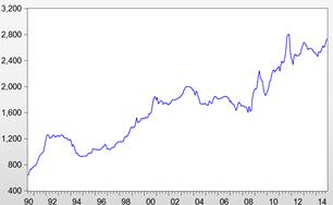
Figure 1. UGDO.
4. Results and Discussion
The time plot of the realization referred to herein as UGDO in Figure 1 shows an overall positive secular trend which indicates a comparative depreciation of the UGX. An initial inspection reveals that annual minimums tend to fall into the first half of the year and the maximums in the later half which is an indication of yearly seasonality. The ADF test statistic value for UGDO is -0.72 and the 1%, 5% and 10% critical values are respectively equal to -3.45, -2.87 and -2.57 respectively. That means the UGDO is adjudged non-stationary. A twelve-monthly differencing of UGDO yields SDUGDO which shows an overall horizontal trend (See Figure 2). With a test statistic value of -3.36, at 1% level of significance, SDUGDO is adjudged as non-stationary also. Its correlogam of Figure 3 attests to its non-stationary nature also. Non-seasonal differencing of SDUGDO yields the series DSDUGDO which also has a flat trend (See Figure 4) and with a test statistic value of -6.00 is certified as stationary by the ADF test. Its correlogram of Figure 5 shows an ACF and PACF suggestive of two models: a SARIMA(0, 1, 1)x(0, 1, 1)12 and a SARIMA(0, 1, 1)x(1, 1, 1)12.
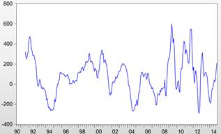
Figure 2. SDUGDO.
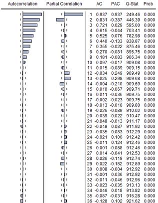
Figure 3. Correlogram of SDUGDO.
Figure 4. DSDUGDO.
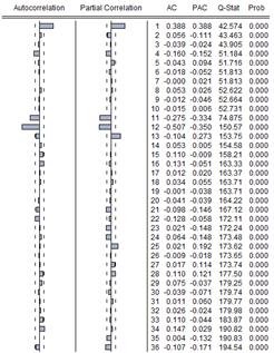
Figure 5. Correlogram of DSDUGDO.
Figure 6. Residual------- Actual-------- Fitted----------.
Figure 7. Correlogram of the sarima (0,1,1)x(0,1,1)12 residuals.
The former model is estimated in Table 1 as
Xt = et + 0.3719et-1 – 0.9382et-12 – 0.3519et (4)
(±0.0560) (±0.0148) (±0.0545)
The latter is estimated in Table 2 as
Xt – .0469Xt-12 = et + .3525et-1 – .9372et-12 - .3344et-1(5)
(±.0630) (±.0589) (±.0152) (±.0567)
Model (4) is the better model in the minimum AIC, Schwarz criterion and Hannan-Quinn criterion sense. The fitted model agrees closely with the data as shown in Figure 6. The correlogram of its residuals in Figure 7 attests to the model adequacy as all the autocorrelations are not statistically significant.
Table 1. Estimation of the sarima(0,1,1)X(0,1,1)12 model. Dependent Variable: DSDUGDO Method: Least Squares.
| Variable | Coefficient | Std. Error | t-Statistic | Prob. |
| MA(1) | 0.371899 | 0.056043 | 6.635904 | 0.0000 |
| MA(12) | -0.938189 | 0.014832 | -63.25510 | 0.0000 |
| MA(13) | -0.351858 | 0.054460 | -6.460897 | 0.0000 |
| Akaike info criterion 10.25209 | ||||
| Schwarz criterion 10.29103 | ||||
| Hannan-Quinn criter 10.26771 | ||||
Table 2. Estimation of the sarima(0,1,1)X(1,1,1)12 model. Dependent Variable: DSDUGDO Method: Least Squares.
| Variable | Coefficient | Std. Error | t-Statistic | Prob. |
| AR(12) | -0.046916 | 0.063016 | -0.744501 | 0.4572 |
| MA(1) | 0.352482 | 0.058892 | 5.985225 | 0.0000 |
| MA(12) | -0.937184 | 0.015190 | -61.69678 | 0.0000 |
| MA(13) | -0.334361 | 0.056735 | -5.893380 | 0.0000 |
| Akaike info criterion 10.26490 | ||||
| Schwarz criterion 10.31850 | ||||
| Hannan-Quinn criter 10.28643 | ||||
5. Conclusion
It has been demonstrated that monthly UGX –USD exchange rates follow a SARIMA(0,1,1)x(0,1,1)12 model. Forecasting of the series may therefore be based on it.
References
- Abdul-Aziz, A. R., Anokye, M., Kwame, A., Munyakazi, L. and Nsowah-Nuamah, N. N. N. (2013). Modeling and Forecasting Rainfall Pattern in Ghana as a Seasonal Arima Process: The Case of Ashanti Region. International Journal of humanities and Social Science, 3(3): 224 – 233.
- Akaike, H. (1977). On Entropy Maximazation Principle. Proceedings of the Symposium on Applied Statistics. (P. R. Krishnaiah, ed.) Amsterdam, North-Holland.
- Asamoah-Boaheng, M. (2014). Using SARIMA to forecast Monthly Mean Surface Air Temperature in the Ashanti Region of Ghana. International Journal of Statistics and Applications, 4(6): 292 – 298.
- Bank of Uganda (2009). Quarterly Economic Report, September, Kampala: BOU.
- Barungi, B. M. (1997). Exchange rate policy and inflation: The case of Uganda. AERC Research Paper 59, African Research Consortium, Nairobi, March.
- Box, G. E. P. and Jenkins, G. M. (1976). Time Series Analysis, Forecasting and Control, Holden-Day, San Francisco.
- Dureval, D., Leoning, J. L., and Birru, Y. A. (2012). Inflation Dynamics and Food prices in Ethiopia. Mimieo.
- Etuk, E. H. (2014). An additive SARIMA Model for Daily Exchange Rates of the Malaysian Ringgit (MYR) and Nigerian Naira (NGN). International Journal of Empirical Finance, 2(4): 193 – 201.
- Etuk, E. H. and Igbudu, R. C. (2015). Appropriate Marketing Information System tools for citrus plantation in Lattakia, Syria: a revisitation. Journal of Multidisciplinary Engineering Science and Technology, 2(1): 180 – 184.
- Etuk, E. H. and Mohamed, M. (2014). Time Series Analysis of Monthly Rainfall data for the Gadaref rainfall station, Sudan, by Sarima Methods. International Journal of Scientific Research in Knowledge, 2(7): 320 – 327.
- Gikungu, S. W., Waititu, A. G. and Kihoro, J. M. (2015). Forecastiing inflation rate in Kenya using SARIMA model. American Journal of the Theoritical and Applied Statistics, 4(1): 15 – 18.
- Hannan, E. J. and Quinn, B. G. (1979). The Determination of the Order of an Autoregression. Journal of the Royal Statistical Society, Series B, 41, 190 – 195.
- Jagathnath, K. K. M., Nithujanathan, V. S., Giriyappa, K. and Chandramouli, D. (2013). Identification of SARIMA as a model for forecasting Indian Leather Export. International Journal of Research in Management, 3(6): 18 – 30.
- Mahsin, M., Akhter, Y. and Begun, M. (2012). Modeling Rainfall in Dhaka Division of Bangladesh Using Time Series Analysis. Journal of Mathematical Modelling and Application, 1(5): 67 – 73.
- Meshran, D. T., Gorantiwar, S. D., Singh, N. V. and Pal, R. K. (2014). SARIMA for generation and forecasting of pomegranate (Punica granatum L.) evapotranspiration of Solapur district of Maharashtra, India. 2nd International Conference on Agricultural & Horticultural Sciences, Radisson Biu Plaza Hotel, Hyderabad, India, February 03 – 05, 2014. www.amicsgroup.org/journals/2168-9881/2168-9881-51.007-082.pdf.
- Otu, A. O., Osuji, G. A., Opara, J., Mbachu, H. I. and Iheagwara, A. I. (2014). Application of Sarima Models in Modelling and Forecasting Nigeria’s Inflation Rates, American Journal of Applied Mathematics and Statistics, 2(1): 16 – 28.
- Pattranurakyothin, T. and Kumnungkit, K. (2012). Forecasting Model for Para Rubber’s Export sales. KMITL Sci. Tech. J., 12(2): 198 – 202.
- Schwarz, G. (1978). Estimating the dimension of a model. Annals of Statistics, 6, 461 – 464.
- Smolen, H. J. (2014). Development of an Influenza Outbreak Forecasting Model Using Time Series Analysis methods, presented at the Pharmacoeconomics and Outcomes Research (ISPOR), 17th Annual European Congress, 8 – 12 November 2014. www.ispor.org/research_pdfs/48/pdffiles/PRM102.pdf
- Suleman, N. and Sarpong, S. (2011). Modeling the Pattern of Reserve Money Growth in Ghana. Current Research Journal of Economic Theory, 4(2): 39 – 42.


