
International Journal of Life Science and Engineering, Vol. 1, No. 1, March 2015 Publish Date: Apr. 2, 2015 Pages: 20-25
A Forecasting Model for Monthly Nigeria Treasury Bill Rates by Box-Jenkins Techniques
Ette Harrison Etuk1, *, Azubuike Samuel Agbam1, Bartholomew Anuriobi Uchendu2
1Department of Mathematics/Computer Science, Rivers State University of Science and Technology, Port Harcourt, Nigeria
2Department of Mathematics/Statistics, Federal Polytechic, Nekede, Imo State, Nigeria
Abstract
A realisation, TBR, of Nigeria Treasury Bill Rates from January 2006 to December 2014 is analysed by seasonal ARIMA methods. The time plot of the realisation reveals an overall downward trend from 2006 to 2009 followed by an overall upward trend up to 2013. Twelve-monthly differencing of TBR yields the series SDTBR which has an overall upward trend. Non-seasonal differencing of SDTBR yields the series DSDTBR with an overall horizontal trend and no clear seasonality. By the Augmented Dickey-Fuller Unit Root Test both TBR and SDTBR are adjudged non-stationary whereas DSDTBR is adjudged stationary. The correlogram of DSDTBR has a negative significant spike in the autocorrelation function at lag 12, an indication of seasonality of period 12 months and the presence of a seasonal moving average component of order one. By a novel proposal credited to Suhartono, initially the (0, 1, 1)x(0, 1, 1)12 SARIMA model is fitted. The non-significance of the lag 13 coefficient suggests the additive SARIMA model with significant coefficients at lags 1 and 12. This model is fitted and has been shown to be the more adequate model and may be used to forecast future Nigeria Treasury Bill Rates.
Keywords
Nigeria Treasury Bill Monthly Rates, SARIMA Models, Additive Models, Time Series, ARIMA Models
Received: March 17, 2015
Accepted: April 1, 2015
Published online: April 2, 2015
@ 2015 The Authors. Published by American Institute of Science. This Open Access article is under the CC BY-NC license. http://creativecommons.org/licenses/by-nc/4.0/
1. Introduction
Many economic and financial time series are known to be seasonal as well as volatile. For instance, crude oil prices, inflation rates, foreign exchange rates, crude oil domestic production are a few such series. Seasonal time series may be modelled using seasonal autoregressive moving average (SARIMA) techniques. Nigeria Treasury Bill Rates constitute such a time series. The purpose of this write-up is to model these rates by SARIMA methods.
Nigeria Treasury Bill is a short-term debt instrument given out by the Federal Government of Nigeria through the Central Bank of Nigeria (CBN) to provide short-term funding for the government (Cashcraft Asset Management Limited, 2013). It is risk-free and re-discountable through licensed Money Market Dealers (Balogun, 2013). The rates are determined by the CBN according to market realities.
Further descriptions of this facility include the following. It is a short-term negotiable bill of exchange, used by government to fund national borrowing requirements, quoted for purchase and sale in the secondary market on an annual percentage yield to maturity and issued at a discount. Its features further include being at zero coupon rate, that is, no interest is paid during the tenure of the bill, being issued in fixed tenures of one-fold, two-fold and four-fold multiples of 91 days. Primary dealers and investment may underwrite it and the interest is paid upfront. Benefits accruable include the fact that they are regarded as liquid assets for the purpose of liquidity ratio calculation and interest received on it is not taxable.
A few examples of such use of the SARIMA methodology to model economic and financial data include the following. Saz(2011) highlighted the comparative advantage of using SARIMA models in terms of parsimony and the efficiency of data modelling. Etuk et al. (2012) modelled Nigerian monthly inflation rates by such methods too. Otu et al. (2014) fitted a SARIMA(1, 1, 1)x(0, 0, 1)12 model to Nigeria’s inflation rates and used it to forecast the series up to 2014. Luo et al. (2013) fitted a SARIMA(1, 0, 1)x(1, 1, 1)12 model to cucumber market prices in China. Dan et al. (2014) fitted a SARIMA(1, 1, 1)x(0, 0, 1)12 model to malaria mortality in Imo State. Lee et al. (2008) were able to observe the superiority of the SARIMA method over two other methods, a neural-based method and a Bayesian based one. Eni and Adesola (2013) fitted a SARIMA(1, 1, 0)x(1, 0, 1) to predict the future volume of traffic from Cross Lines Limited, a transport Company. Osarunwense (2013) fitted a SARIMA(0, 0, 0)x(2, 1, 0) model to quarterly rainfall data in Port Harcourt. Teye-Okutu (2011) fitted a SARIMA(1, 1,1,1)x(0,0,1)12 and used it to forecast Ghanaian inflation. Monthly precipitation in Mount Kenya region has been modelled as a SARIMA (1,0,1)x(1,0,0)12 by Kibunja et al. (2014).
Where seasonal series are involved they have been observed to exhibit comparative advantage (see for instance Lee et al. (2008)). It is noteworthy that most fitted SARIMA models are multiplicative as defined by Box and Jenkins (1976). For instance all the above-mentioned works applied multiplicative models. Box and Jenkins (1976) however considered the possibility of a non-multiplicative such model. They did not define an additive SARIMA model.
It is Suhartono (2011) and Suhartono and Lee (2011) that defined a subset, multiplicative and additive SARIMA model. Using airline data Suhartono observed that the subset model outdid the additive one. However with the tourist arrival to Bali data, the additive model displayed some supremacy over the subset model. Suhartono and Lee (2011) observed that the additive model outdid the others in terms forecasting the number of tourist arrivals at Bali. Both works aimed at proposing a new algorithm for SARIMA fitting. This algorithm shall be considered in detail in the methodology section. The SARIMA models fitted by Etuk et al. (2013) and Etuk et al.(2014) to monthly Nigerian Naira-CFA Franc Exchange Rates and Monthly Nigerian Savings Deposit Rates respectively turned out to be additive.
2. Methodology
The data for this work are monthly Nigeria Treasury Bill Rates from January 2006 to December 2014 retrievable from the Money Market Indicators, Data and Statistics publication of the CBN in its website www.cenbank.org.
2.1. Sarima Models
A stationary time series {Xt} is said to follow an autoregressive moving average model of orders p and q, designated ARMA(p, q), if it satisfies the following difference equation
![]() (1)
(1)
where {et} is a white noise process and the a’s and b’s are constants such that the model is both stationary and invertible. Model (1) may be written as
A(L)Xt = B(L)et (2)
where A(L) = 1 - a1L - a2L2 - ... - apLp and B(L) = 1 + b1L + b2L2 + ... +bqLq and L is the backward shift operator defined by LkXt = Xt-k.
Most real life time series are non-stationary. Box and Jenkins(1976) proposed that differencing to a sufficient order could render a non-stationary time series stationary. Suppose the series {Xt} is non-stationary. Let d be the minimum order such that the dth difference of Xt , namely, ÑdXt, is stationary where Ñ = 1 - L. Stationarity may be tested using Augmented Dickey-Fuller(ADF) Unit Root Test. If the series {ÑdXt} follows an ARMA(p, q) the original series {Xt} is said to follow an autoregressive integrated moving average model of orders p, d and q designated ARIMA(p, d, q).
For a seasonal time series of order s, Box and Jenkins(1976) proposed that {Xt} be modelled by
![]() (3)
(3)
where the series must have been subjected to seasonal differencing D times and non-seasonal differencing d times, Ñs = 1 – Ls, being the seasonal differencing operator. Moreover F(L) and Q(L) are the seasonal autoregressive and moving average operators respectively. These seasonal operators are polynomials in L. Suppose that F(L) = 1 + f1L + f2L2 + ... +fPLP and Q(L) = 1 + q1L + q2L2 + ... + qQLQ then the time series {Xt} is said to follow a multiplicative seasonal autoregressive integrated moving average model of orders p, d, q, P, D, Q and s, designated (p, d, q)x(P, D, Q)s SARIMA model.
Suhartono(2011), using moving average (MA) symbolism, defines a subset SARIMA model as
![]() (4)
(4)
where bs+1 ¹ b1bs. Otherwise, it is a multiplicative SARIMA model. If bs+1 = 0, the model (4) is said to be an additive SARIMA model. He goes on to propose the following set of steps for SARIMA fitting:
1) Fit a subset SARIMA model.
2) Find out if bs = 0. If so, the model is additive. If not, find out if the model is multiplicative. If not, the model is subset.
2.2. Model Estimation
In order to fit the model (3) the orders p, d, q, P, D, Q and s must first be determined. Often seasonality is not evident from the time plot. After due differencing a spike in the autocorrelation function (ACF) and often in the partial autocorrelation function (PACF) indicates seasonality of period equal to the corresponding lag s. In order to avoid undue model complexity it has been advised that d + D < 3. Most often it is allowed that d= D=1. The non-seasonal autoregressive order p is estimated by the non-seasonal cut-off lag of the PACF and q by the non-seasonal cut-off lag of the autocorrelation function ACF. The seasonal orders P and Q are respectively determined by the seasonal cut-off lags of the PACF and ACF.
The parameters of the model are invariably estimated by non-linear optimization techniques because of the involvement of items of the white noise process in the model. An initial estimate of the parameters is usually made and on its basis further estimates are obtained iteratively, each estimate expected to be an improvement on its predecessor until optimality is attained depending on the degree of accuracy required. The optimality criterion employed is usually the least squares criterion, the maximum likelihood criterion, the maximum entropy criterion, etc.
After model fitting analysis of the residuals is usually done with a view to ascertaining the adequacy of the model. This is called diagnostic checking. Assuming model adequacy the residuals should have zero mean, be uncorrelated and follow a Gaussian distribution. In this write-up all analytical work is done using the Eviews 7 software which uses the least squares approach to estimation. Besides Eviews 7 displays values of three information criteria on the basis of which model comparison could be done. The information criteria are Akaike Information criterion (AIC) (Akaike, 1977), Schwarz information criterion (Schwarz, 1978) and Hannan-Quinn information criterion (Hannan and Quinn, 1979). A low criterion value is an indication of relative model adequacy.
3. Results
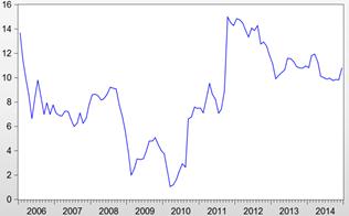
Figure 1. TBR
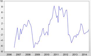
Figure 2. SDTBR
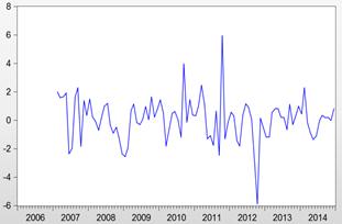
Figure 3. DSDTBR
The time plot of the realization TBR in Figure 1 reveals an overall negative trend between 2006 and 2009, followed by an overall positive trend from 2010 onwards. Regular seasonality is not obvious. However an inspection of the data reveals that yearly minimums occur in May, July, December, February, March, July, December, February and September respectively. That means that six of the nine minimums lie between February and July of the same year. Similarly, five of the nine maximums lie in the remaining part of the year. This is an indication of a 12-monthly seasonality. This justifies a SARIMA modelling approach.
A twelve-month differencing of this original series yields the series SDTBR which has an overall slightly upward trend with no observable regular seasonality as evident from Figure 2. A non-seasonal differencing results in the series DSDTBR which shows no trend on the overall and no clear seasonality (See Figure 3). The ADF unit root test statistic for TBR, SDTBR and DSDTBR is equal to -1.9, -2.4 and -8.6 respectively. With the 1%, 5% and 10% critical values equal to -3.5, -2.9 and -2.6 respectively, the ADF test adjudges both TBR and SDTBR non-stationary but DSDTBR stationary. In the correlogram of DSDTBR in Figure 4, there is a negative significant spike at lag 12 in the ACF. This shows that the series is seasonal of period 12 months. Moreover, this is an indication of the presence of a seasonal MA component of order one.
Adopting Suhartono’s (2011) set of steps, a (0, 1, 1)x(0, 1, 1)12 SARIMA model fit yields the model (5) as summarized in Table 1:
![]() (5)
(5)
Clearly the lag 13 coefficient is non-significant. Hence the model is additive which is re-estimated as summarized in Table 2 as
![]() (6)
(6)
which is clearly superior to model (5) on the grounds of the minimum of the information criteria: Akaike information criterion, Schwarz information criterion and Hannan-Quinn information criterion. The adequacy of model (6) is evident from
1) The close agreement of the fitted model and the actual model (See Figure 5).
2) The uncorrelatedness of the residuals as seen from their correlogram of Figure 6. None of the 36 autocorrelations is significant (i.e. outside of the range ±2/Ön, where n is the sample size).
4. Conclusion
It may be concluded that Nigeria Treasury Bill Rates follow the additive SARIMA model (6). That means that a current value of the time series depends on the past value of a month ago and that of a year ago of shocks or its error terms. This model has been shown to be adequate and could be used for the forecasting of Nigeria treasury Bill rates. However efforts should be made to explore the possibility of models that better account for the variability in the time series.
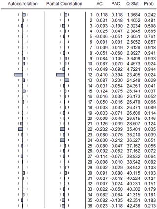
Figure 4. Correlogram of Dsdtbr
Table 1. (0, 1, 1)X(0, 1, 1)12 Sarima Model Estimation
Dependent Variable: DSDTBR Method: Least Squares
| Variable | Coefficient | Std. Error | t-Statistic | Prob. |
| MA(1) | 0.154011 | 0.102767 | 1.498643 | 0.1374 |
| MA(12) | -0.916250 | 0.030967 | -29.58813 | 0.0000 |
| MA(13) | -0.123210 | .103857 | -1.186342 | 0.2385 |
| Akaike info criterion 2.956466 Schwarz criterion 3.0337114 Hannan-Quinn criter. 2.989054 | ||||
| Inverted MA Roots ±.99, .86±.50i, .49±.86i, ±.99i, -0.13, -.50±.86i, -.86±.50i | ||||
Table 2. Additive Sarima Model Estimation
Dependent Variable: DSDTBR Method: Least Squares
| Variable | Coefficient | Std. Error | t-Statistic | Prob. |
| MA(1) | 0.042042 | 0.037105 | 1.133043 | 0.2601 |
| MA(12) | -0.916117 | 0.030681 | -29.85973 | 0.0000 |
| Akaike info criterion 2.951810 Schwarz criterion 3.005576 Hannan-Quinn criter. 2.973535 | ||||
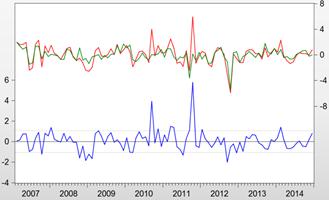
Figure 5. ---- Residual ---- Actual ---- Fitted
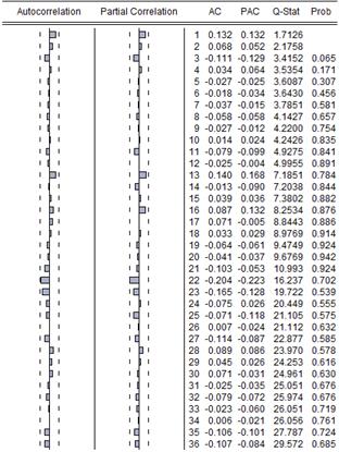
Figure 6. Correlogram of the Residuals of the Additive Sarima Model
References
- Akaike, H. (1977). "On Entropy Maximization Principle:" Proceedings of the Symposium on Applied Statistics (P. R. Krishnaiah, ed.) Amsterdam, North-Holland.
- Balogun, M. (2013). "Understanding the Nigerian Treasury Bills Market", www.ipledge2nigeria.com/index.php/blogs/entry/understanding-the-nigerian-treasury-bills-market.html
- Box, G. E. P. and Jenkins, G. M. (1976)."Time Series Analysis, Forecasting and Control", Holden-Day, San Francisco.
- Cashcraft Asset Management Limited (2013). "Treasury Bills", www.cashcraft.com/index.php?option=com_content&view=article&id=3448&Itemid=157
- Dan, E. D., Jude, O., Idochi, O. (2014). Modelling and Forecasting Malaria Mortality rate Using SARIMA Models (A Case Study of Aboh Mbaise General Hospital, Imo State, Nigeria), Science Journal of Applied Mathematics and Statistics, 2(1), 31-41.
- Eni, D. and Adesola, A. W. (2013). Sarima Modelling of Passenger Flow at Cross Line Limited, Nigeria. Journal of Emerging Trends in Economics and Management Sciences (JETEMS), 4(4), 427-432.
- Etuk, E. H., Aboko, I. S., Victor-Edema, U., Dimkpa, M. Y. (2014). An Additive Seasonal Box-Jenkins model for Nigerian monthly savings deposit rates. Issues in Business Msanagement and Economics, 2(3), 54-59.
- Etuk, E. H., Asuquo, A. and Essi, I. D. (2012). "Seasonal Box-Jenkins Model for Nigerian Inflation Rate Series", Journal of Mathematical Research, 4(4), 107-113.
- Etuk, E. H., Wokoma, D. S. A. and Moffat, I. U. (2013). Additive Sarima Modelling of Monthly Nigerian Naira-CFA Franc Exchange Rates. European Journal of Statistics and Probability, 1(1), 1-12.
- Hannan, E. J. and Quinn, B. G. (1979). "The Determination of the Order of an Autoregression."Journal of the Royal Statistical Society, Series B, 41, pp. 190-195.
- Kibunja, H. W., Kihoro, J. M., Orwa, G. O., Yodah, W. O. (2014). Forecasting Precipitation Using SARIMA model: A Case Study of Mt. Kenya Region. Mathematical Theory and Modeling, 4(11), 50-58.
- Lee, K. J., Chi, A.Y., Yoo, S. Jin, J. J. (2008). Forecasting Korean Stock Price Index (KOSPI) using back propagation neural network model, Bayesian Chio’s model, and SARIMA Model. Allied Academies International Conference, 249-252.
- Luo, C. S., Zhou, L. Y. and Wei, O. F. (2013). Application of SARIMA Model in Cucumber Price Forecast, Applied Mechanics and Materials, 373-375, 1686-1690.
- Osarunwense, O. (2013). Applicability of Box-Jenkins SARIMA model in rainfall Forecasting: A Case study of Port Harcourt South South Nigeria. Canadian Journal on Computing in Mathematics, Natural sciences, Engineering and Medicine, 4(1), 1-4.
- Otu, A. O., Osuji, G. A., Opara, J. Mbachu, H. I., Iheagwara, A. I. (2014). Application of Sarima Models in Modelling and Forecasting Nigeria’s Inflation Rates. American Journal of Applied Mathematics and Statistics, 2(1), 16-28.
- Saz, G. (2011). "The Efficacy of SARIMA Models for Forecasting Inflation Rates in Developing Countries: The case for Turkey."International Research Journal of Finance and Economics, 62, 111-142.
- Schwarz, G. (1978). "Estimating the Dimension of a model." Annals of Statistics, 6, pp. 461-464.
- Suhartono (2011). "Time Series Forecasting by using Autoregressive Integrated moving Average: Subset, Multiplicative or additive Model." Journal of Mathematics and Statistics, 7(1), 20-27.
- Suhartono and Lee, M. H. (2011). "Forecasting of Tourist Arrivals Using Subset, Multiplicative or Additive Seasonal ARIMA Model", Matematika, 27(2), 169-182.
- Teye-Okutu, E.M.K. (2011). Modelling and Forecasting Ghana’s inflation rates using Sarima models. A Thesis submitted to the Department of Mathematics, Kwame Nkrumah University of Science and Technology in partial fulfilment of the requirements for the award of M.Sc. in Industrial Mathematics.


