Technology Applications of the Low Drag Shapes of Aquatic Animals

Igor Nesteruk^*

Institute of Hydromechanics, National Academy of Sciences of Ukraine, Kyiv, Ukraine

Abstract

The best swimmers have a streamlined shape that ensures an attached flow pattern even in the case of inertial motion (without varying the body shape). Similar rigid bodies of revolution were calculated and tested in the wind tunnel. In the middle of the body, the measured static pressure is significantly higher than the theoretical values. The influence of this fact on the boundary layer separation was estimated. In order to explain the discrepancy in experimental and theoretical pressure distributions, some inverse problems were solved.

Keywords

Drag Reduction, Boundary Layer Separation, Flow Control, Aquatic Animals

Received: April 10, 2015
Accepted: May 1, 2015
Published online: May 27, 2015

@ 2015 The Authors. Published by American Institute of Science. This Open Access article is under the CC BY-NC license. http://creativecommons.org/licenses/by-nc/4.0/

1. Introduction

The high swimming velocities of some aquatic animals continue to amaze the researches, since the density of water is approximately 800 times greater than the density of air. The corresponding values of the Reynolds number  (is the velocity of movement, is the length of the body,  is the kinematic viscosity coefficient) exceed ten millions (e.g., in the case of dolphin) and are typical for the turbulent boundary layer on the body surface. The friction drag of the dolphin, estimated with the use of turbulent friction coefficient of the flat plate, [1], was so great to declare that the dolphin should not be able to swim as fast as it does with the muscle power it possesses. Gray proposed to solve the paradox that the dolphin must reduce drag by maintaining a laminar flow in the boundary layer about its body, delaying the transition to turbulence by movements of its tail, [1]. Discussion of the question has continued over the seven decades since it was advanced; after Gray, further ideas have been put forward involving possible drag-reducing properties of dolphin skin ranging from dermal ridges to skin compliance and to dermal secretions.

In addition, testing the rigid bodies, similar to the animal shapes, [2], and gliding animals (during the inertial movement without a manoeuvring and a shape change, [3]), was carried out in order to explain the fact of the low drag by a very good shape only. From the point of view of these researches, their experiments reveal flow patterns without boundary layer separation. On the other hand, the researches connected with industrial application believe that separation is inevitable at any rigid body (if any active flow control methods such as suction etc. are applied). Their conviction it based on a commonly adopted practice to aim the static pressure minimum to coincide with the maximum of the body radius, which leads to a positive pressure gradient and a separation downstream of this point, [4]. In this paper, we will focus on this contradiction and will provide a new analysis of experimental results.

First, the theory does not restrict a body to have negative pressure gradients both up- and downstream of the maximum thickness point. In particular, some examples of axisymmetric shapes with pressure decreasing near the tail have been calculated with the use of both the ideal and the viscous fluid approaches (e.g., [5,6]); and manufactured and tested in wind tunnels [7,8]. Unfortunately, a pressure decrease near the body tail is not enough to remove separation. For example, the flow separated on Goldschmied’s body; the separation was removed only with the use of suction.

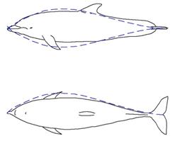
Fig. 1. Comparison of the shape UA-2c with the body of a bottlenose dolphin

The special shaped bodies of revolution with negative pressure gradients have been calculated and tested in [9-11]. An example - shape UA-2c - is shown in Fig. 1. Other examples of special axisymmetric shapes with different diameter to length ratio D/L are shown in Fig. 2. Both the forebody and the tail of the shape corresponding to the smallest thickness ratio =0.1, are concave, while for less slender bodies (=0.21 and =0.3) only the tail is concave (see Fig. 2). Some fast-swimming fish have a concave forebody too (e.g., the Mediterranean spearfish Tetrapturus belone, Indo-Pacific sailfish Istiophorus platypterus, black marlin Makaira indica , or swordfish Xiphias gladius).

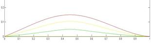
Fig. 2. Examples of slender bodies of revolution () with negative pressure gradients near the trailing edge, Calculations with the use of the exact solution of the Euler equations proposed in [8-10].

2. Research Significance

Elongated unseparated shapes of the best swimmers allow reducing the pressure drag. According to the d’Alembert paradox its value tends to zero at large Reynolds numbers. In addition, the attached boundary-layer remains laminar on the slender bodies of revolution at rather large Reynolds numbers and the critical value of the Reynolds number increases with the diminishing of the thickness ratio D/L, see [11,12]. Thus, the attached air- and hydrodynamic shapes are of obvious practical interest, since they allow reducing their drag and noise.

3. The Shape of the Test Body and Support Sting. Theoretical and Experimental Pressure Distributions

During last 20 years the possibility of achieving a laminar attached flow on a rigid body was investigated in the Institute of Hydromechanics (IHM) of National Academy of Sciences, Kyiv, Ukraine. The survey of these theoretical and experimental studies is presented in [10]. For this study, we take the model UA-2, which is an unclosed version of the shape UA-2c shown in Fig.1. Both shapes were calculated from the exact solution of Euler equations. By a special distribution of the sources and sinks on the axis of symmetry, the stream function of the axisymmetric potential flow of the inviscid incompressible fluid was represented as follows, [9,10]:

  (1)

, ,

,  ,

Where  are cylindrical coordinates. The corresponding axisymmetric body radius , flow components ,  and pressure coefficient on the surface were calculated with the use of following equations:

, , ,          (2)

Varying the values of parameters  different closed shapes can be obtained, in particular those shown in Figs. 1 and 2.

To fix the model on the wind tunnel we need a support tube, which could be also simulated by the exact solution (1), (2), since the parameters  allow changing the balance of the sinks and the sources. A result of the calculations – shape UA-2 – is shown in Fig.3. Solid black and blue lines represent the body radius and corresponding pressure distribution respectively. Downstream to the point   the body radius diminishes very slowly and  is close to zero.

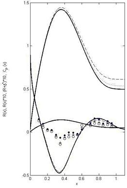
Fig. 3. Unclosed shape UA-2

Radius and pressure coefficients (solid black and blue lines) are calculated from (1), (2) The laminar unseparated boundary layers at Re_L =90 000 and Re_L =700 000 and corresponding pressure distributions are shown by dashed and dotted lines respectively. The lengths are based on the model length L=200 mm. Experimental static pressure measurements [9,10] are shown by markers (dots, crosses and circles for Re_L =90 000; 150 000; 240 000 respectively).

The test model UA-2 is of 200 mm length and 56.78 mm of the maximum diameter. For the experiments, downstream to the point  the calculated shape was replaced by the cylindrical support tube of the 300 mm length and 19.98 mm external diameter.

To estimate the displacement thickness of the laminar boundary layer on the model and support sting the following formula can be used, [10,13]:

                     (3)

Formula (3) follows from the Blasius solution for the plane plate and the Mangler-Stepanov transformations (see [14]) and is valid for the slender bodies of revolution () and when . The calculations at Re_L =90 000 and Re_L =700 000 are shown in Fig. 3 by dashed and dotted black lines respectively.  The exact solution (1), (2) allows finding the shapes which at  are very close to the new shapes with the  radius and calculating the corresponding pressure distributions. The results are shown in Fig. 3 by blue dashed and dotted lines for Re_L =90 000 and Re_L =700 000 respectively.

Very small differences in theoretical pressure distributions at Re_L >90 000 allow expecting the same experimental results, if the real boundary layer remains attached and laminar. In the experiments [9,10] a very significant discrepancy between the experimental und theoretical pressure distributions was revealed, especially in the middle part of the body (see Fig. 3). Nevertheless, no visible separation and turbulence zones (e.g., the reversed flows) were revealed in tests with the use of the wire probe, [9,10].

The same facts were revealed in experiments with the use of rigid bodies similar to the aquatic animals’ shape, [2] . For example, the values of the pressure coefficient, measured on the shapes similar to the tuna’s (Thunnus alalunga) and dolphin’s (Delphinus delphis ponticus Barab.) ones, were no less than -0.17 (see [2] , Table 12). The minimum theoretical values of the pressure coefficients on the corresponding axisymmetric bodies with the same values of D/L (0.21-0.22) are less than -0.4. It must be noted, that such significant discrepancy between the experimental data and the expected minimal values of the pressure coefficient exists even at rather high Reynolds numbers, e.g., in the experimental values of  Re_L  were 6.3-6.9 millions.

In the next Sections we will analyze the in influence of the real pressure distribution on the boundary layer separation and will try to find the corresponding shapes.

4. Estimations of the Laminar Boundary Layer Separation

To analyze the influence of the real and theoretical pressure distributions on separation, the following criterion was used for the point of laminar separation on the body of revolution, [15] :

   (4)

Where  is the velocity of the inviscid flow at the outer edge of the boundary layer. Using (4) and the theoretical pressure distribution from the exact solution (1), (2) yields the value  for the position of the laminar separation line on the body UA-2.

The same criterion (4) was applied for the experimental pressure distributions. The linear interpolation of the experimental   data allows calculating  and its derivative. The calculations show that possible separation lines are located downstream to the point  at all Reynolds numbers of IHM experiments. On the other hand, at   the experiments revealed the pressure recovery and rather good agreement with the theoretical line (see Fig.3). This fact makes the separation unlikely.

5. Solutions of the Inverse Problems

In order to analyze which shapes correspond to experimental pressure distributions some inverse problems were solved. The exact solution (1), (2) was modified by adding doublets distributed on the axis of symmetry. The corresponding intensities of the doublets were calculated to fit the experimental pressure data. The results of calculations are presented in Figs. 4 and 5. The experimental data at Re_L=2.4*10⁵ from [9,10] were used (shown by markers).

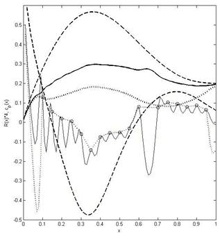
Fig. 4. Shapes (4*R(x), back lines) corresponding to different pressure distributions (blue lines).

Shape UA-2 and its theoretical pressure distribution (exact solution (1), (2)) are shown by dashed lines. Solid lines show the solution of the inverse problem with the use of doublets located at the points of static pressure measurements. Dotted lines represent the solution of the inverse problem with the use of doublets located at a distance of 0.01 apart and linear interpolation of the experimental data at Re=2.4*10⁵ shown by markers.

If the doublets are located only in the points of the static pressure measurements, the corresponding pressure distribution and shape are rather irregular (solid lines). With the doublets located at a distance of 0.01 apart and the linear interpolation of the experimental data, the corresponding dotted lines become smoother. However, in both cases the corresponding shapes are significantly different from the body UA-2 (dashed line). In the areas  and , the corresponding pressure distributions are very different (see blue solid and dotted lines in Fig. 4).

The attempts to find a solution of the inverse problem trying to fit the experimental pressure data and real body radius revealed no convergence. The solution of the inverse problem with the partial use of the experimental data (e.g., the odd points only) may yield better agreement with the real body shape and theoretical pressure distribution (compare solid and dashed lines in Fig. 5). Probably, the reason of the discrepancy in the theoretical and experimental pressure distributions may be some unsteady structures in the flow.

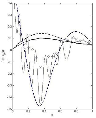
Fig. 5. Shapes (back lines) corresponding to different pressure distributions (blue lines). Shape UA-2 and its theoretical pressure distribution (exact solution (1), (2)) are shown by dashed lines. Solid lines show the solution of the inverse problem with the use of doublets located at the odd points of the static pressure measurements.

6. Conclusions

The significant difference in the theoretical (corresponding to the inviscid potential flow) and experimental pressure distributions on the special shaped body UA-2 (and similar shapes of best swimmers) can be a reason of the attached boundary layer. The solutions of the inverse problems obtained with the use of the experimental static pressure data yield the shapes, which are very different from the real body UA-2. The further theoretical investigation may be focused on the searching of unsteady structures in the flow. Further experiments are necessary with the use of different flow visualization methods, in particular, application the hot-wire velocity probes to clarify the behavior of the boundary layer, its separation and laminar-to-turbulent transition characteristics.

Acknowledgements

The author thanks Alberto Redaelli, Giuseppe Passoni and Gianfranco Fiore (Politecnico di Milano) for their support and interesting discussion of the results.

The study was supported by EU-financed project EUMLS (EU-Ukrainian Mathematicians for Life Sciences) - grant agreement PIRSES-GA-2011-295164-EUMLS

References

1. Gray, J. 1936 Studies in animal locomotion VI. The propulsive powers of the dolphin. J. Exp.Biol. 13, 192-199.
2. Aleyev, Yu. G. Nekton. Dr. W. Junk, The Hague, 1977.
3. Rohr, J., Latz, M. I., Fallon, S., and Nauen, J. C. Experimental approaches towards interpreting dolphinstimulated bioluminescence. J. Exper. Biology 201: 1447–1460, 1998.
4. L.D. Landau, E.M. Lifshits, Fluid Mechanics, Second Edition: Volume 6 (Course of Theoretical Physics), Butterworth-Heinemann, 1987.
5. Zedan, M.F., Seif,A.A. & Al-Moufadi, S. Drag Reduction of Fuselages Through Shaping by the Inverse Method. J. of Aircraft 31, No. 2: 279-287. 1994
6. Lutz, Th. & Wagner, S. Drag Reduction and Shape Optimization of Airship Bodies. J. of Aircraft. 35, No. 3: 345-351, 1998.
7. Goldschmied, F.R.  Integrated hull design, boundary layer control and propulsion of submerged bodies: Wind tunnel verification. In AIAA (82-1204), Proceedings of the AIAA/SAE/ASME 18th Joint Propulsion Conference, pp. 3–18, 1982.
8. Nesteruk, I. Experimental Investigation of Axisymmetric Bodies with Negative Pressure Gradients. Aeronautical J. 104: 439-443, 2000.
9. Nesteruk, I. New type of unseparated subsonic shape of axisymmetric body. Reports of the National Academy of Sciences of Ukraine, 11: 49-56, 2003 (in Ukrainian).
10. Nesteruk, I. Rigid Bodies without Boundary-Layer Separation. Int. J.of Fluid Mechanics Research,41, No. 3: 260-281, 2014.
11. I. Nesteruk, G. Passoni, A. Redaelli. "Shape of Aquatic Animals and Their Swimming Efficiency," Journal of Marine Biology, vol. 2014, Article ID 470715, 9 pages, 2014. doi:10.1155/2014/470715.
12. Nesteruk, I. Peculiarities of Turbulization and Separation of Boundary-Layer on Slender Axisymmetric Subsonic Bodies. Naukovi visti, NTUU "Kyiv   Polytechnic Institute" 3, 70-76. 2002.(in Ukrainian).
13. I. Nesteruk, Reserves of the hydrodynamical drag reduction for axisymmetric bodies,Bulletin of Univ. of Kiev, Ser.: Phys. & Math. 4 (2002) 112-118.
14. L.G. Loitsyanskiy. Mechanics of Liquids and Gases, Begell House, New York and Wallingford, 6th ed, 1995.
15. Kwang S. Hyun, Paul K. Chang. The criterion of separation of incompressible laminar boundary layer flow over an axially symmetric body.JJ. of the Franklin Institute, v.325, Issue 4, 1988, pp. 419–433.